Quick Answer
A 50,000 m² automotive parts factory in Pune runs 24 hours a day, 6 days a week, with three rotating shifts and a 4 MW connected load. The roof can host 3.2 MWp of solar. The plant manager assumes a 3.2 MWp array will offset 80 percent of the bill.
A 50,000 m² automotive parts factory in Pune runs 24 hours a day, 6 days a week, with three rotating shifts and a 4 MW connected load. The roof can host 3.2 MWp of solar. The plant manager assumes a 3.2 MWp array will offset 80 percent of the bill. The actual offset, after a year of operation, is 41 percent. Why? Because half the plant’s energy use happens at night, the noon production curve overshoots daytime demand by 28 percent, and the local utility pays 0.04 USD/kWh for export against a 0.14 USD/kWh purchase rate. This is the central design problem of factory solar, and getting it right has nothing to do with picking better panels.
A 50,000 m² automotive parts factory in Pune runs 24 hours a day, 6 days a week, with three rotating shifts and a 4 MW connected load. The roof can host 3.2 MWp of solar. The plant manager assumes a 3.2 MWp array will offset 80 percent of the bill.
TL;DR — Factory Solar System Design
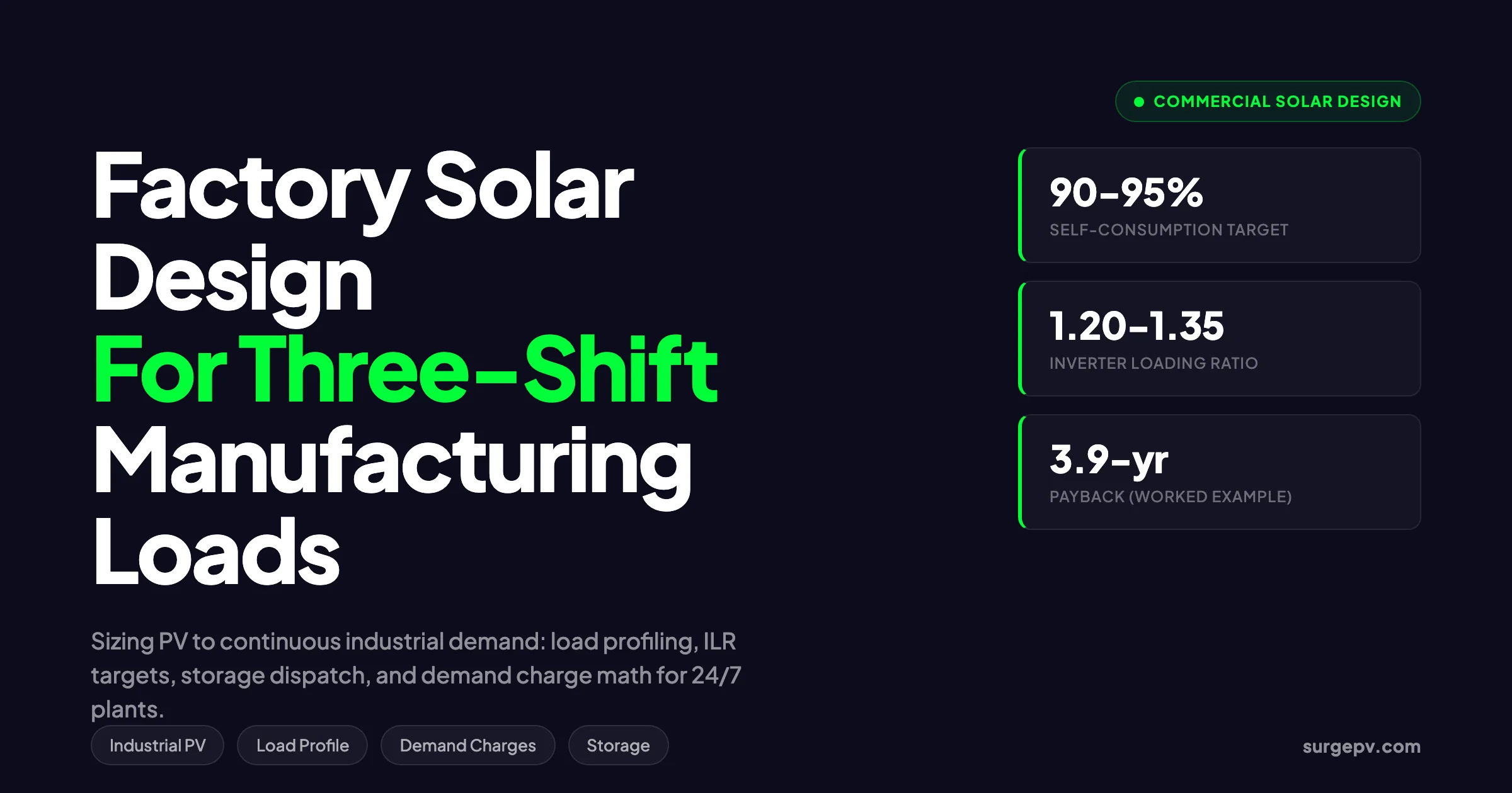
For three-shift continuous manufacturing, size the array to the daytime baseline load (typically 50 to 70 percent of nameplate connected load), not the rooftop area. Use 15-minute interval data for 12 months, target an ILR of 1.20 to 1.35, and add storage only if demand charges exceed 15 USD/kW or TOU spreads exceed 0.10 USD/kWh. Average self-consumption above 90 percent is the real KPI, not capacity factor.
This guide covers the full design workflow for matching photovoltaic generation to three-shift manufacturing loads, with concrete numbers from real factory deployments, the load profile analysis methodology, sizing math, inverter and storage decisions, and the financial models that separate factories where solar pays back in five years from those where it stretches to ten.
What Makes Factory Solar Different From Other Commercial PV
Most commercial solar guides describe a building that runs from 8 AM to 6 PM, five days a week — offices, retail, schools, warehouses with daytime distribution. The energy profile is a flat plateau from 9 to 5, with weekend troughs. Solar fits that shape beautifully, and a properly sized array on a 9-to-5 building can self-consume 70 to 85 percent of generation.
A factory running three rotating shifts is a different animal. Production lines do not stop. HVAC systems serving cleanroom or process-controlled environments run 24 hours. Compressed air, chilled water, and process water loops are continuous. Lighting drops between shifts but never goes to zero. The result is a load profile that looks like a slightly wavy plateau across the entire 168-hour week, with shift-changeover bumps every eight hours and brief Sunday morning troughs during weekly maintenance windows.
This load shape changes every assumption in commercial PV design. The capacity factor of the building matters less than the daytime-to-nighttime ratio of consumption. The peak load metric matters less than the load floor. Demand charges matter more than energy charges. And the standard tools used to design commercial PV — sized to peak demand, optimized for capacity factor, modeled against a typical commercial load shape — produce systems that overgenerate at noon and undergenerate during shift transitions.
Pro Tip
Before any sizing math, request 12 months of 15-minute interval data from the factory’s smart meter. If the utility cannot provide it, install a temporary class-1 power meter on the main incomer for a minimum of 30 days. Sizing factory solar without interval data is the most common cause of underperforming industrial PV.
The discipline matters because a poorly sized factory array does not just underperform — it actively destroys value. Every kWh exported at 0.04 USD instead of self-consumed at 0.14 USD is a 0.10 USD lost per unit. A 3 MWp array that exports 25 percent of its annual generation in a low-feed-in market loses approximately 110,000 USD per year compared to a 2.2 MWp array that self-consumes 95 percent.
Load Profile Analysis: The Foundation of Factory Solar
Every factory PV design starts with one artifact: a 12-month, 15-minute-interval log of plant-level kW demand. This is the load profile and it tells you everything that matters before a single panel layout is drawn.
What the Load Profile Reveals
Five metrics extract from interval data:
Daytime baseline (kW) — The 25th percentile of demand between 09:00 and 16:00, averaged across weekdays. This is what your solar array can serve without exporting.
Daytime average (kW) — The mean demand between 09:00 and 16:00, weekdays only. Typically 10 to 30 percent above the daytime baseline.
Daytime peak (kW) — The 95th percentile of the same window. Used for inverter and switchgear sizing, not array sizing.
Nighttime average (kW) — Mean demand between 22:00 and 05:00. For a true three-shift factory, this should be 60 to 90 percent of the daytime average. If it is below 50 percent, the plant is not actually running three full shifts.
Weekend ratio — Saturday and Sunday daytime average divided by weekday daytime average. A continuous-process factory will be 0.85 to 1.0. A 6-day operation drops to 0.40 to 0.60 on Sundays. This is the single biggest predictor of weekend export risk.
Reading a Three-Shift Profile
A typical three-shift factory load profile looks like this:
| Time Window | Typical Load (% of plant peak) | What’s Running |
|---|---|---|
| 22:00 – 05:00 (Night shift) | 70-85% | Production lines, continuous chillers, compressed air, base lighting |
| 05:00 – 06:00 (Shift change) | 90-100% | Both shifts overlap, all utilities at full draw |
| 06:00 – 14:00 (Day shift) | 95-105% | Full production, peak HVAC load, full office lighting |
| 14:00 – 15:00 (Shift change) | 95-100% | Overlap, slight bump |
| 15:00 – 22:00 (Evening shift) | 85-95% | Production continues, HVAC tapers |
The shift-change overlaps are critical. Many factories run a 30 to 60 minute crossover where outgoing and incoming workers are both on the floor, equipment is being handed over, and machinery is checked. During these overlaps, the plant momentarily approaches its connected load capacity. A solar array sized to the daytime average will undersupply during these windows, which is fine — the grid covers the gap. A solar array oversized to the peak will dump excess to grid during the calmer mid-shift hours, which is expensive.
The 15-Minute vs Hourly Trap
A common mistake is using monthly utility bills (kWh totals) or hourly averaged data to design factory solar. Both miss the granularity that matters. A factory with a peak demand charge structure pays based on the highest 15-minute average each month. Hourly data smooths out the actual peaks, which means PV-plus-storage designs based on hourly data systematically underdeliver on demand charge reduction.
For a deeper treatment of this, see our guide on solar system sizing using 15-minute interval load data.
Sizing Methodology: From Load Profile to Array Size
Once you have clean 15-minute interval data, sizing follows a five-step process.
Step 1: Establish the Daytime Energy Pool
Sum the kWh consumed between 06:00 and 18:00, weekdays only, for 12 months. This is your daytime energy pool. For a 4 MW factory running three shifts, this typically falls between 8.5 and 11 GWh per year (out of a total annual consumption of 25 to 32 GWh).
Step 2: Set the Self-Consumption Target
For factory solar in 2026, target 90 to 95 percent self-consumption. This means at most 5 to 10 percent of solar generation is exported. The math:
Maximum array generation = Daytime energy pool ÷ self-consumption target
                        = 9.5 GWh ÷ 0.92
                        = 10.3 GWh per year
Step 3: Convert kWh to kWp Using Specific Yield
Specific yield (kWh per kWp per year) varies by climate. Approximate values for industrial belts:
| Region | Specific Yield (kWh/kWp/year) |
|---|---|
| Northern Germany / UK Midlands | 950 - 1,050 |
| Pune / Mumbai (India) | 1,500 - 1,650 |
| Texas Gulf Coast / Northern Mexico | 1,650 - 1,800 |
| Southern Spain / Greece | 1,700 - 1,850 |
| Riyadh / Dubai | 1,850 - 2,000 |
| Shenzhen / Bangkok | 1,350 - 1,500 |
For our Pune factory:
Optimal array size = 10.3 GWh ÷ 1,550 kWh/kWp/year
                   = 6,645 kWp DC
This is the maximum size that maintains 92 percent self-consumption. The actual installed size depends on roof availability, capex constraints, and grid export rules.
Step 4: Validate Against Roof Area
A bifacial 600 Wp module occupies approximately 2.4 m² (panel area plus row spacing for tilt-mounted designs, slightly more for ballasted flat-roof systems). A 6.6 MWp array therefore needs: Read Bifacial Solar Panel Design Guide for a complete walkthrough.
Roof area required = 6,645 kWp ÷ 0.6 kWp per panel × 2.4 m² per panel
                   = 26,580 m²
Most automotive or pharma factories of 4 MW connected load have 40,000 to 60,000 m² total roof, of which 60 to 70 percent is usable after subtracting skylights, HVAC mounts, fire setbacks, and structural exclusion zones. Roof area is rarely the binding constraint for factories of this scale — load profile is. Also see: Us Residential Solar Market Trends 2026.
Step 5: Validate Against Grid Connection Limits
Many countries cap behind-the-meter solar at the contracted demand or at a fixed percentage of it. India limits net-metered C&I solar to the contracted load. Germany requires a separate study for systems above 1 MW. Mexico’s Generación Distribuida regime caps at 0.5 MW; above that, the system must be classified as Generación Limpia Distribuida or an off-take arrangement. For the latest details on India, see 5kW Solar Panel Price in India.
For deeper coverage of export limit regimes, see our guide on grid export limitation rules by country.
Inverter and DC/AC Ratio Design for Continuous Loads
The inverter loading ratio (ILR) — DC array kWp divided by inverter AC kW — is one of the most consequential design choices in factory PV.
Why Factories Want Higher ILR Than Generic Commercial
A standard commercial PV design uses an ILR of 1.10 to 1.20. The logic: keep clipping minimal, maximize annual yield per dollar of inverter. For factories with continuous daytime loads above the inverter’s AC rating, this logic flips.
When ILR is increased from 1.15 to 1.30, three things happen:
- Noon production gets clipped slightly — losses of 1 to 3 percent annually.
- Morning and afternoon production rises — energy harvest expands by 2 to 5 minutes on each side of the day.
- The fixed inverter cost serves more panels — capex per kWh drops by 6 to 10 percent.
For a factory whose daytime load substantially exceeds the inverter’s AC output, the clipping at noon does not matter — the plant absorbs every AC kW the inverter produces, and clipped DC kW would have been exported at low rates anyway. The shoulder-hour gain is pure self-consumption uplift.
Pro Tip
For three-shift factories with a daytime average load above 1.5x the planned inverter AC rating, target an ILR of 1.30 to 1.40. The clipping loss is more than offset by improved utilization of the daytime load envelope. Use solar design software that simulates clipping at 15-minute resolution against your actual load profile, not annual averages.
Inverter Selection: String vs Central
Three factors push factory PV toward central inverters above 1 MWp:
- Roof segments are large and uniform — a 30,000 m² metal-deck roof is the natural fit for 100 to 250 kW string inverters or 1 to 3 MW central inverters.
- Reactive power capability matters — central inverters typically offer wider Q ranges (cos φ from 0.8 leading to 0.8 lagging) compared to string inverters at 0.9 leading to 0.9 lagging.
- Single point of MV connection — factories already operate at 11 kV or 33 kV, and central inverters with integrated step-up transformers simplify the interconnection.
String inverters win when:
- The roof has multiple orientations or is segmented by skylights and equipment platforms.
- The factory wants modular fault tolerance (a single string failure takes 100 kW offline, not 1 MW).
- The interconnection is at LV (400 V or 480 V) and the array is below 1.5 MWp.
For factories above 2 MWp on monolithic roofs, central inverters reduce capex by 0.05 to 0.08 USD/Wp. For factories below 1 MWp or with complex roofs, string inverters break even or come out ahead.
Storage: When and How Much
Battery storage is the most overspecified component in factory solar design. Many proposals add storage by default, sized to “support critical loads” or “provide backup.” For most three-shift factories, the right answer is no storage, or a small storage system targeted exclusively at demand charge reduction. Read Adding Battery Storage Services for a complete walkthrough.
When Storage Makes Sense
Storage on a factory PV system pays back in three scenarios:
Scenario 1 — High demand charges. If the demand charge component of the bill is above 15 USD/kW per month (or local equivalent), peak shaving with a 1 to 2 hour battery can shift the billing peak off the daytime curve. A 500 kW / 1 MWh battery can flatten a 200 to 300 kW peak demand spike, saving 40,000 to 70,000 USD per year on a 1 MW factory.
Scenario 2 — Time-of-use spreads above 0.10 USD/kWh. Markets with TOU tariffs that price peak hours (typically 17:00 to 21:00) above 0.20 USD/kWh and off-peak below 0.10 USD/kWh create arbitrage opportunities. The battery charges during midday solar peak and discharges during the evening tariff peak.
Scenario 3 — High export curtailment penalties or near-zero feed-in tariffs. Where grid export is curtailed above a certain percentage of contracted demand, storage absorbs the would-be-curtailed energy and discharges it during night-shift consumption.
Sizing Storage for Three-Shift Factories
Unlike residential or commercial solar where storage covers the evening peak after the building closes, factory storage rarely covers night-shift load — that would require a battery 4 to 8 times larger than the financial model supports. Instead, factory storage is sized to either:
Demand charge reduction — Battery capacity in kWh equals the highest peak event duration (in hours) times the peak shaving target (in kW). A factory with a 200 kW peak lasting 90 minutes needs roughly 300 kWh of usable energy plus 20 percent for round-trip efficiency and depth-of-discharge limits, giving 360 to 400 kWh nameplate.
Self-consumption uplift on Sundays — A Sunday-only off-shift schedule creates 8 to 12 hours of low load. A battery sized to 30 to 40 percent of Sunday peak production captures the would-be export and dispatches it Monday morning before solar ramps up.
For a comprehensive treatment of how to size storage in commercial settings, see our guide on commercial battery storage sizing.
LFP vs NMC for Industrial Storage
Lithium iron phosphate (LFP) chemistry has won the industrial storage segment. The reasoning:
| Factor | LFP | NMC |
|---|---|---|
| Cycle life (80% DoD) | 6,000 - 10,000 | 3,000 - 5,000 |
| Thermal runaway threshold | 270°C | 210°C |
| Cost per kWh (system) | 280 - 380 USD | 320 - 450 USD |
| Energy density (Wh/kg) | 90 - 120 | 150 - 220 |
For industrial use cases, the energy density penalty does not matter — a battery in a parking-lot container has unlimited footprint compared to an EV. The cycle life advantage is decisive: a factory cycling once daily for 365 days a year for 10 years runs 3,650 cycles, comfortably inside LFP’s working envelope and at the upper end of NMC’s.
Designing factory solar at scale?
SurgePV simulates 15-minute load profiles against your array layout, models inverter clipping with shift-by-shift accuracy, and runs storage dispatch optimization for demand charge and TOU arbitrage in a single workspace.
Book a DemoNo commitment required · 20 minutes · Live project walkthrough
For a direct comparison, see Arka 360 vs SurgePV.
Roof Considerations for Industrial PV
Factory roofs come in three structural classes, each with distinct PV implications.
Metal Deck (Standing Seam or Trapezoidal)
The dominant roof type for modern factories. Standing seam roofs accept clamp-on rail systems with no roof penetrations, preserving warranty. Trapezoidal profiles require either standing seam adapters or hanger bolts through the rib peak.
Structural capacity: typically 15 to 20 kg/m² superimposed dead load. A 20 kg/m² PV system (rails + modules + cable) is at the upper limit. Bifacial modules at 600 Wp weigh approximately 13 kg/m² of mounted area, leaving 5 to 7 kg/m² for racking.
Wind uplift is the engineering risk on metal-deck roofs. For tilt angles above 5°, dynamic loading from wind on the upwind row can exceed the clip-to-deck attachment rating. A standard rule: limit tilt to 5° on standing seam, 10° on trapezoidal with through-deck fasteners, and engage a structural engineer for anything above. See our flat roof ballasted solar systems guide for a detailed treatment.
Concrete Slab
Common in older factories and warehouses. Higher dead load capacity (30 to 80 kg/m²) but expensive penetrations and waterproofing risk push designs toward ballasted systems.
Ballasted designs need a slope analysis and a wind tunnel study (or accepted CPP/RWDI report) for tilts above 10°. Typical ballast adds 30 to 60 kg/m², which combined with module weight pushes total load to 45 to 75 kg/m². Pre-ballast structural review is mandatory.
Asbestos Cement Sheet
Common in factories built before 2000. PV mounting is technically possible but creates hazardous material handling complexity. The recommended path is roof replacement before solar installation. Many EPCs bundle the two: replace asbestos sheet with insulated metal panel, then install PV. The roof replacement cost is partially offset by avoided future demolition liability.
Power Quality and Reactive Power Compensation
A frequently overlooked factor in factory PV design: the inverter’s ability to supply reactive power.
The Power Factor Problem
Industrial loads are heavily inductive. Motors, transformers, and discharge lighting all consume reactive power, pushing the plant power factor below the 0.95 threshold most utility tariffs require. Plants below the threshold pay penalties; some markets impose charges per kVAr above the limit.
Traditional factories install capacitor banks for PF correction. These are passive, sized for average reactive demand, and switched in steps. They cannot follow rapid changes in motor load.
How Solar Inverters Replace Capacitor Banks
A modern grid-tied PV inverter is a 4-quadrant device: it can deliver real power (P) and supply or absorb reactive power (Q) simultaneously. Most central inverters specify Q capability of cos φ 0.8 to 1.0 (lagging) and 1.0 to 0.8 (leading), even at full P output. Many can supply Q without P (at night, when the array is dark) up to 50 percent of nameplate kVA.
This means a 1 MW solar inverter at a factory can:
- Generate 1,000 kW of real power during sunshine, while simultaneously supplying 200 kVAr of reactive power for PF correction.
- At night, supply 500 kVAr of reactive power, replacing a portion of the capacitor bank.
For a factory paying 25,000 USD per year in PF penalties, the avoided capacitor bank capex (50,000 to 150,000 USD) plus avoided penalties make the inverter PF capability one of the most undermarketed wins in factory solar.
Configuration Notes
PF correction requires:
- Inverter firmware that supports Q-V or fixed cos φ control modes.
- A communication link to the plant SCADA or to the main incomer meter.
- A control logic that prioritizes P export during the day and Q during shoulder/night hours.
Not all inverters offer this out of the box. Specify it in the tender.
Tariff Structures and Their Design Impact
Three tariff structures dominate factory solar economics globally, and each pushes the design in a different direction. For Global-specific compliance details, see Global net-metering-by-country.
Time-of-Use Energy Charges
Energy charges differ by hour of day, typically with a peak block (afternoon and evening), a shoulder block (morning and late evening), and an off-peak block (overnight). Spain’s industrial tariffs are a clean example, with six time periods and peak rates 4 to 6 times higher than off-peak. For the latest details on Spain, see Hotel Solar + EV Charging Case Study. For Spain-specific information, see Solar Panels Spain.
Design implication: PV is most valuable during peak and shoulder hours. East-west split arrays with morning and afternoon production peaks outperform south-facing arrays in markets with bimodal peak periods. See our guide on east-west vs south-facing solar layouts.
Demand Charges (kW)
Demand charges bill the highest 15-minute or 30-minute average power draw each month. A factory with a 2 MW peak and a 20 USD/kW/month demand charge pays 480,000 USD per year just on capacity, regardless of energy consumed.
Design implication: Solar must reliably reduce the billed peak. A 3 MWp array on a clear day at noon helps. The same array on an overcast Tuesday afternoon does not — and the billed peak is set on the worst day, not the average. Storage is the only reliable peak-shaving asset for demand charges.
Maximum Demand or Capacity Charges
Common in Europe and parts of Asia. The contracted demand (in kVA) sets the maximum simultaneous load and the corresponding fixed monthly charge. Exceeding contracted demand triggers penalties or contract upgrades. Also see: European Solar Incentives.
Design implication: Solar that reduces utility-supplied demand can support a contracted demand reduction at contract renewal — converting a one-time tariff renegotiation into 5 to 10 years of fixed-charge savings. Quantify this and include it in the solar proposal software output.
For factories in Europe, our guide on solar self-consumption rules across Europe covers how each country structures the financial model.
A Worked Sizing Example: 4 MW Pune Auto Parts Factory
To make the methodology concrete, here is a complete worked example for a real factory archetype.
Plant Profile
| Parameter | Value |
|---|---|
| Industry | Automotive component manufacturing |
| Connected load | 4,000 kW |
| Contract demand (kVA) | 4,400 |
| Operating schedule | 24 hours, 6 days/week, 50 working weeks/year |
| Annual consumption | 27,500,000 kWh |
| Daytime (06:00-18:00) consumption | 14,200,000 kWh (52%) |
| Weekday daytime baseline | 2,150 kW |
| Weekday daytime peak (95th percentile) | 3,200 kW |
| Weekend daytime average | 1,800 kW (Saturday), 850 kW (Sunday) |
| Tariff (HT industrial) | 0.105 USD/kWh energy + 5.2 USD/kVA demand |
| Net metering | Capped at 1 MW; above that, net billing at 0.045 USD/kWh export |
| Roof | 32,000 m² metal deck, standing seam, ~70% usable after exclusions |
Sizing Calculation
Daytime energy pool (weekdays + Saturday): 14.2 GWh
Self-consumption target: 92%
Maximum self-consumed solar generation: 14.2 ÷ 0.92 = ~13.05 GWh net of array losses (we’ll target 13 GWh AC delivered)
Specific yield in Pune: ~1,575 kWh/kWp/year for fixed-tilt south-facing bifacial array on metal deck
Array size for 13 GWh: 13,000 ÷ 1,575 = 8,254 kWp
Roof constraint: 32,000 × 0.70 = 22,400 m² usable. At 2.4 m² per 600 Wp panel, 9,333 panels = 5,600 kWp. Roof binds.
Net metering constraint: 1,000 kWp eligible for net metering. Above this, export rate falls to 0.045 USD/kWh.
Final array size: 5,600 kWp — limited by roof, with the first 1 MW under net metering.
Inverter Configuration
- AC rating: 4,400 kW (ILR 1.27)
- Topology: 6 × 800 kW central inverters with integrated MV step-up to 11 kV
- Reactive power capability: ±0.8 cos φ at full P, ±0.5 Q at zero P (night)
- Estimated noon clipping: 2.1% of annual DC production
Annual Production and Self-Consumption
- DC generation: 5,600 × 1,575 = 8,820 MWh
- AC delivered (after 96% inverter efficiency, 2.1% clipping, 1% AC losses): 8,150 MWh
- Daytime energy pool weekdays + Saturday: 14,200 MWh — solar fits within
- Sunday daytime production: approximately 230 MWh per year exported (3% of generation)
Financial Outcome
| Line | Value (USD) |
|---|---|
| Capex (5.6 MWp at 0.62 USD/Wp installed in India 2026) | 3,472,000 |
| Year 1 self-consumed energy savings (7,920 MWh × 0.105) | 831,600 |
| Year 1 export revenue (230 MWh × 0.045) | 10,350 |
| Year 1 PF correction savings | 22,000 |
| Year 1 demand charge offset (estimated 8% reduction at margin) | 18,300 |
| Year 1 total benefit | 882,250 |
| Simple payback | 3.9 years |
| 25-year NPV at 8% discount, 3% tariff escalation | 9.1M |
This is the financial profile that makes factory solar one of the most reliable industrial energy investments in 2026.
Battery Time-Shift Modeling for Factories with Demand Charges
For factories where demand charges dominate the bill (common in the US, parts of Mexico, and South Africa), battery time-shift modeling becomes the central design exercise. The methodology: For Africa-specific compliance details, see Africa solar compliance.
Step 1 — Identify the Top 5% of Demand Events
From 12 months of 15-minute data, extract the highest-demand events. For a 2 MW factory, these are typically the moments when production lines, HVAC, and compressed air all reach simultaneous peak — often during the morning shift starting at 06:00 or during a summer afternoon at 14:00.
Step 2 — Quantify Peak Shaving Value
For each high-demand event, calculate:
Peak shaving value = (event peak kW - 90th percentile baseline kW) × demand charge rate × 12 monthsIf the top 12 events average 350 kW above baseline at a 22 USD/kW demand charge, peak shaving value = 350 × 22 × 12 = 92,400 USD/year.
Step 3 — Size the Battery to the Event
For events lasting 1.5 hours at 350 kW peak shaving:
Battery energy required = 350 kW × 1.5 hours ÷ (round-trip efficiency × usable DoD)
                       = 525 kWh ÷ (0.92 × 0.90)
                       = 634 kWh nameplate
Battery power rating: 350 kW continuous, 400 kW for short-duration peaks.
Step 4 — Validate Solar-Charged vs Grid-Charged
A battery charged from solar adds revenue stream (avoided export at low rate). A battery charged from off-peak grid creates pure tariff arbitrage. Most factory designs use a hybrid dispatch: solar-charge during the day when surplus exists, grid-charge overnight from off-peak hours when needed for next-day peak coverage.
Real Numbers
A 350 kW / 700 kWh LFP battery in 2026 costs approximately 250,000 USD installed. Against 92,400 USD annual savings, payback is 2.7 years. Stack this onto a solar payback of 4 to 5 years and the combined system pays back in approximately 4.2 years.
Compressed Air, Chillers, and HVAC: The Hidden Solar Leverage
Three load categories dominate factory energy use. Each interacts with solar differently.
Compressed Air
A typical manufacturing plant runs compressors at 25 to 35 percent of total electricity consumption. Compressors are largely steady-state — they cycle on and off but the duty cycle is consistent across shifts. This makes compressed air an ideal solar match: the load is daytime-heavy (production-tied), the demand profile is predictable, and short interruptions are tolerable.
Air receivers act as natural mechanical storage. A factory with a 50 m³ receiver at 8 bar can ride through 60 to 90 seconds of compressor downtime. This means a momentary cloud passage that drops solar output is masked by the receiver, eliminating one of the operational concerns of variable PV power.
Chillers and Process Cooling
Chiller loads correlate with ambient temperature. Summer afternoon chiller demand peaks exactly when solar production peaks — a fortunate coincidence for sizing.
A chiller with thermal storage (an ice tank or chilled water tank) extends this match. The chiller runs at maximum capacity during solar peak, freezing water or cooling a tank, then runs at reduced capacity during shift changes when solar dips. Thermal storage is 5 to 10 times cheaper per kWh than battery storage for cooling-only applications.
HVAC
HVAC loads correlate with both ambient and occupancy. Three-shift factories have flat occupancy 24/7, so HVAC is more weather-driven than shift-driven. Solar matches well during cooling season (summer), poorly during heating season (winter, when most HVAC demand is at night).
In mixed-climate factories, HVAC alone is rarely the dominant solar argument. It is one of several daytime loads that solar covers efficiently.
Roof Mounting Methods for Industrial-Scale Arrays
The choice of mounting system on a factory roof determines installation speed, structural risk, and long-term maintenance access.
Clamp-On Standing Seam
Best for: standing seam metal roofs in good condition. Pros: No penetrations, fast installation (4 to 6 kWp per crew per day), preserves roof warranty. Cons: Limited tilt angles (typically 5° max), sensitive to wind uplift, requires confirmed seam profile compatibility.
Through-Deck Fasteners on Trapezoidal
Best for: trapezoidal profile metal roofs with good substrate condition. Pros: Allows higher tilts (10° to 15°), proven structural attachment, accepts varied panel layouts. Cons: Roof penetrations require flashing, slower installation, slight risk to long-term watertightness if not properly sealed.
Ballasted on Concrete Slab
Best for: flat concrete roofs with sufficient structural capacity. Pros: No penetrations, reversible installation, allows deeper tilt (10° to 15°), faster install on simple geometry. Cons: Heavy (45 to 75 kg/m² total), requires structural review, restricted to flat or near-flat substrates, ballast can shift over time.
Tensioned Cable Systems
Best for: sawtooth or arched factory roofs with high vertical clearance. Pros: Adapts to non-flat geometries, can be installed without scaffolding, suspended panels avoid roof contact entirely. Cons: Specialized engineering, higher capex, niche supplier base.
For most modern factories with metal-deck roofs, the choice is between clamp-on standing seam and through-deck on trapezoidal. The seam profile and the roof age determine which fits.
Working with Long-Term Power Purchase Agreements
For factories with strong creditworthiness, a third-party-owned PPA can convert a 3 to 5 million USD capex into an off-balance-sheet operating expense.
How Industrial PPAs Work
A renewable energy developer or financier installs, owns, and operates the array. The factory commits to purchase the solar output for 15 to 25 years at a fixed (or escalator) rate, typically 10 to 30 percent below the current grid rate.
When PPAs Make Sense
- Factory has weak balance sheet capex availability or competing capital priorities.
- Tax structure does not reward direct asset ownership (no investment tax credit, no accelerated depreciation benefit).
- Factory wants to lock in a fixed energy rate to hedge tariff increases.
- Operations and maintenance is outside core competency.
When PPAs Don’t Make Sense
- Factory has strong access to capex at 6 to 8 percent rates and long planning horizon.
- Local depreciation or tax incentives favor direct ownership (India’s 40% accelerated depreciation, US ITC + MACRS, etc.).
- Factory is not creditworthy enough to attract competitive PPA pricing.
- Factory plans relocation within the PPA term.
A self-financed system in India with accelerated depreciation typically delivers a 15 to 18 percent IRR. A PPA on the same factory typically delivers 8 to 12 percent in tariff savings — substantial, but lower than direct ownership.
Common Design Mistakes in Factory Solar
Across hundreds of industrial PV designs, the same mistakes recur.
Sizing to Roof Area Instead of Load
Engineers see a 40,000 m² roof and propose 5 MWp because the roof “supports it.” For a 2 MW factory with a daytime baseline of 1.4 MW, a 5 MWp array exports 50 to 60 percent of generation at low rates. The right size for that factory is 1.4 to 1.8 MWp, even if 60 percent of the roof stays empty.
Designing Without 12 Months of Data
Single-month or 3-month load data hides seasonal variation. A factory in a temperate climate may have 30 percent higher summer demand from cooling. A factory in a heating-dominated climate has 40 percent higher winter demand from process heat. Solar that matches summer load oversizes for winter.
Ignoring Process Variability
Factories rarely run at constant production. Order books fluctuate, model changeovers reduce throughput for days at a time, and annual maintenance shutdowns drop load to 5 to 10 percent of normal for one to two weeks per year. A solar design assuming 50 production weeks at 95 percent capacity overestimates self-consumption.
Underspecifying the Inverter Communication Layer
A factory PV system must integrate with plant SCADA, the main incomer meter, and (often) the energy management system. Inverters that ship without Modbus TCP, OPC-UA, or IEC 61850 communication fail at integration and force costly retrofits.
Skipping the Structural Engineer
A 5 MWp rooftop array imposes loads that few existing factory roofs were designed for. Skipping a structural review to save 8,000 to 15,000 USD in engineering fees is the most common cause of post-installation roof damage and warranty disputes.
Conclusion
- Start with 12 months of 15-minute interval data, not roof area or panel count. Every meaningful design decision flows from the load profile.
- Size the array to the daytime baseline, target 90 to 95 percent self-consumption, and only increase size if export economics justify it. For factories above 2 MW connected load, the right array is usually 50 to 70 percent of connected load.
- Add storage only when demand charges or TOU spreads create a clear payback. Defaulting to storage on every project destroys financial returns.
Frequently Asked Questions
How do you size a solar system for a factory running three shifts?
Start with 15-minute interval load data for at least 12 months. Identify the daytime baseline (the load floor between 06:00 and 18:00 across all shifts) and size the PV array to cover 80 to 110 percent of that baseline at noon. Sizing for the daytime average rather than the peak avoids exporting on weekends and during ramp-down periods, which is where most factory solar designs lose money.
Should a factory with continuous production add battery storage?
Only if the tariff has time-of-use rates with a peak-to-off-peak spread above 0.10 USD/kWh, or if demand charges exceed 15 USD/kW per month. Three-shift factories already self-consume most of their solar generation, so the storage payback comes from peak shaving and demand charge reduction, not from time-shifting energy. Without those tariff signals, batteries rarely pencil out.
What is the right inverter loading ratio for a factory rooftop?
Most three-shift factory designs use an ILR between 1.20 and 1.35. Higher ratios push more energy into the morning and afternoon shoulders, when shift changeovers raise process loads. Going above 1.40 starts clipping noon production, which is fine if the noon peak exceeds plant demand, but wasteful if it does not.
How much rooftop space does a factory need for meaningful solar coverage?
A modern bifacial 600 Wp module needs roughly 2.4 m² of clear roof area per panel. A 1 MWp factory rooftop array therefore needs 4,000 m² to 4,500 m² of unshaded, structurally sound roof. Most light-industrial factories with metal-deck roofs can host 30 to 80 percent of their connected load capacity in solar without structural reinforcement. Shadow analysis software identifies shading issues before installation.
Do factory solar systems need to be designed differently for night shifts?
Yes. The system itself is not different, but the financial model is. Night-shift consumption is supplied entirely by the grid regardless of solar size, so the optimization target shifts from generation maximization to daytime self-consumption. This usually means sizing the array smaller than a single-shift retail or office building of the same roof area would justify.
How does a factory’s power factor affect solar design?
Inductive motor loads pull the power factor below 0.95, which raises the apparent power the inverter must serve and triggers PF penalties on most industrial tariffs. Modern string and central inverters can supply reactive power up to roughly 0.90 leading to 0.90 lagging, which means a properly programmed solar inverter can correct PF without a separate capacitor bank. This is one of the largest hidden savings on factory PV.
What payback period is realistic for factory solar in 2026?
Five to seven years is normal for a self-consumption-led design in markets with electricity tariffs above 0.12 USD/kWh. Factories paired with battery storage and demand charge reduction can hit four to six years where peak demand charges exceed 20 USD/kW per month. Export-heavy designs with weak feed-in rates push payback past nine years.
Should a factory with continuous chillers or compressed air systems prioritize solar over efficiency upgrades first?
No. Variable-frequency drives on motors, leak repair on compressed air, and waste heat recovery on chillers usually return 30 to 50 percent energy savings at one-quarter the capital cost of solar. The right sequence is efficiency first, then solar sized to the post-efficiency load. Sizing solar to the inefficient baseline locks in oversized arrays that export at low rates.