Solar System Sizing: 15-Minute Interval Load Data

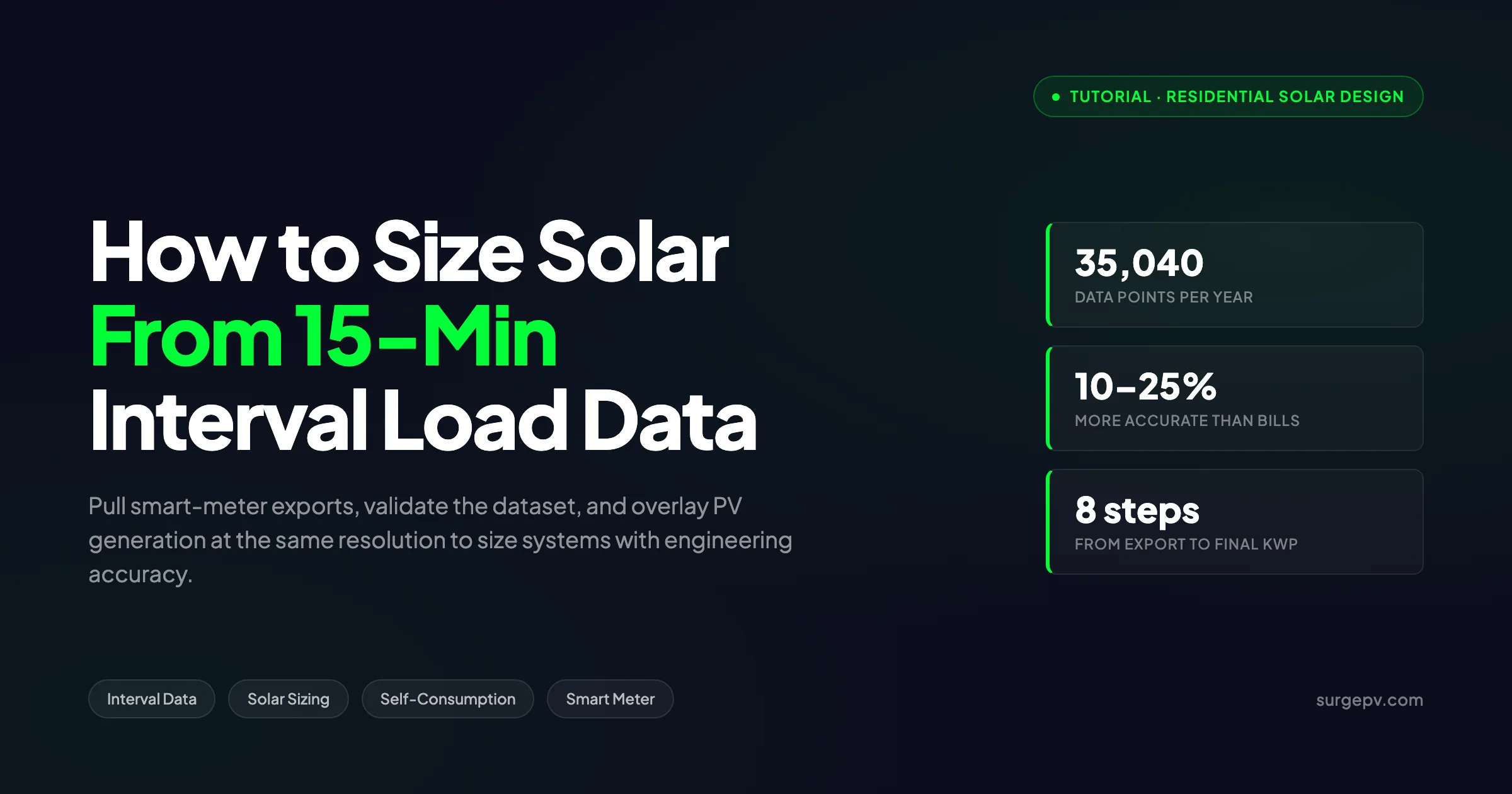
Sizing a solar system from monthly utility bills produces a guess. Sizing it from 15-minute interval load data produces an engineering answer. The difference is roughly 35,040 data points per year versus 12. That granularity separates a system that hits its self-consumption target from one that overshoots, undershoots, or sends much of its output to a low-value export tariff. This tutorial walks through the full workflow: pulling the data from a smart meter, cleaning it, mapping the load shape, overlaying PV generation in the same intervals, and arriving at a system size that survives a tariff audit. The same method works for residential, light commercial, and off-grid sizing once you understand what each interval is telling you.

Last updated: November 2026.

What this guide covers:

1. What 15-minute interval data is and why it beats monthly bills
2. How to pull interval data from a utility smart meter
3. Cleaning, validating, and gap-filling the dataset
4. Aggregating energy and identifying peak demand
5. Mapping the daily and seasonal load profile
6. Simulating PV generation at matching 15-minute intervals
7. Calculating self-consumption rate without and with batteries
8. Iterating kWp to hit the right size for the tariff
9. A worked example with an illustrative 11,420 kWh household
10. Common mistakes that produce undersized or oversized systems

Every section includes the formulas and validation checks you need. The numbers in the examples are illustrative, not measured data.

Why 15-Minute Interval Data Beats Monthly Bills for Solar Sizing

A monthly utility bill compresses 30 days of varying consumption into one number. That number drives the simplest sizing formula every solar designer learns: divide annual kWh by the local yield factor (kWh/kWp/year) and you have your kWp. The formula works for a rough proposal. It fails the moment the project involves time-of-use tariffs, demand charges, batteries, or any meaningful difference between morning and evening usage.

15-minute interval data shows the load shape directly. Each reading is an average kW value for that quarter-hour window, and 35,040 readings span a full year. With that resolution you can see the 6 a.m. spike when the heat pump kicks on, the midday lull while the house is empty, the 5 to 9 p.m. peak when EVs and induction stoves run together, and the gentle overnight baseload. None of this appears in a monthly bill.

The granularity matters because solar production is not uniform either. PV output follows irradiance, which follows the sun, which means generation peaks at solar noon and falls off after 4 p.m. local time. Most residential and commercial loads peak in the morning and evening, when generation is low. The mismatch between these two curves drives every important number in a solar proposal: self-consumption rate, export volume, demand charge reduction, and battery payback.

Working with interval data lets a designer answer questions that monthly bills cannot:

• What percentage of solar generation is consumed directly versus exported?
• How much would a battery shift to evening usage and at what payback?
• Will the system reduce the 15-minute demand charge or just the energy charge?
• Does the load shape justify a tilt or azimuth different from local optimum?
• How much will the system actually save under a time-of-use tariff?

Working With Interval Data to Plan for PV Systems, published by Greentech Renewables, frames the value plainly: PV systems can offset a higher percentage of a customer’s bill than the simple energy fraction implies because production aligns with peak pricing windows. Interval data is the only way to quantify that effect.

What 15-Minute Interval Data Actually Contains

A typical interval data export is a CSV or XML file with three core columns: timestamp, energy or power value, and unit. The energy column is reported either as kWh consumed during the interval or as average kW during the interval. The two are interchangeable through the conversion kWh = kW x 0.25, since each interval is 0.25 hours.

The Green Button Connect standard, used by most US utilities and adopted by several international utilities, encodes interval data as XML with explicit time zone tags, interval length, and unit fields. Utility customer portals such as PG&E’s Download My Data, SCE’s Green Button portal, and SDG&E’s interval data export all produce Green Button-compatible files. Energy Toolbase notes that Green Button data ships in 60, 30, or 15-minute increments depending on the utility.

A clean 15-minute dataset for one year looks like this:

35,040 rows total. Annual consumption is the sum of column three. Peak 15-minute demand is the maximum of column two. Average load is column three divided by 0.25 hours.

For commercial sites, additional columns may appear: reactive power (kVAR), power factor, and demand reading per billing period. For solar sizing the active power column is sufficient. The reactive power data becomes relevant only when sizing reactive power compensation or assessing inverter Q-mode requirements.

How to Get 15-Minute Interval Data From a Smart Meter

The data exists if the customer has an advanced metering infrastructure (AMI) smart meter, which is now standard in most developed markets. The path to obtain it depends on jurisdiction.

United States

Most investor-owned utilities offer self-service exports through the customer portal. The three California utilities lead in coverage:

• Pacific Gas and Electric: Download My Data, available in the energy management section of the customer account. Check the portal for the history length and formats it offers.
• Southern California Edison: Green Button portal at sce.com, check its portal for the history length.
• San Diego Gas and Electric: Energy use details with a download option; check which intervals it offers.

Outside California, ConEd, Duke Energy, Xcel, and PSE&G provide similar exports. Coverage varies. Utilities that have not deployed full AMI may only offer hourly data or daily reads.

For installer workflows, third-party data services such as Utility API, Arcadia, and UtilityScore automate the export with customer authorization. The customer signs a one-page release, the service pulls the data via OAuth, and the installer receives the dataset without chasing the customer.

Europe and the United Kingdom

Smart meter rollouts in the EU and UK followed national plans. Most distribution operators provide half-hourly data, which is the European standard, with some moving to 15-minute resolution under the EU Electricity Market Design framework. Octopus Energy in the UK exposes half-hourly data through its API. In Germany, smart meter gateways can supply quarter-hourly values to authorized users. In Italy, ask the distributor or the customer portal. For wider context on European support schemes, see European solar incentives.

For half-hourly markets, the workflow is identical except each interval is 30 minutes and the year contains 17,520 readings. The conversion to 15-minute resolution requires linear interpolation, which loses some peak granularity but is acceptable for most sizing tasks.

Australia

Australian smart meters record interval data, commonly at 30-minute or 5-minute resolution. Retailers and distributors provide it through customer portals or on request, so ask for the finest resolution available.

Off-Grid and New Builds

For projects without a meter, interval data has to be modeled. Use a reference load shape from a similar building type, scaled to expected annual kWh, and overlay known appliance schedules. Reference building load profiles published by national laboratories, such as NREL’s end-use load profiles for the US building stock, cover most building types. For new homes, the appliance method works: list every appliance with its rated kW and daily run hours, distribute the run hours across the day, and aggregate into 15-minute bins.

Cleaning and Validating the Dataset Before You Size

Raw interval exports are rarely production-ready. Common issues include missing intervals, daylight saving time gaps, time zone errors, unit confusion (kW versus kWh), and duplicate timestamps. Skipping the validation step is the most frequent cause of sizing errors that pass internal review and only surface after the system is built.

Validation Checklist

Run these checks before any sizing math:

1. Row count: A full year of 15-minute data has 35,040 rows in standard time, plus or minus 4 rows for daylight saving transitions. Off by more than 1 percent means missing intervals.
2. Continuous timestamps: Sort by timestamp and confirm that each row is exactly 15 minutes after the previous. Any jump greater than 15 minutes is a gap.
3. Time zone consistency: Confirm the time zone tag matches the project location. Mismatches between meter UTC offsets and PV simulation local time cause irradiance overlap errors.
4. Daylight saving handling: In spring forward, one hour goes missing. In fall back, one hour duplicates. Both need explicit handling, either by interpolating the missing hour or by averaging the duplicates.
5. Unit check: Confirm whether the value column is kW (average power) or kWh (interval energy). Mixing the two produces a 4x error in either direction.
6. Sanity check on totals: Sum the dataset to annual kWh. Compare against the customer’s last 12 utility bills. They should match within 2 percent. Larger gaps indicate missing intervals or unit confusion.

Gap Filling Rules

Short gaps (1 to 4 missing intervals) can be filled by linear interpolation between the surrounding values. Longer gaps require more care:

• Up to 1 hour missing: Linear interpolation.
• 1 to 24 hours missing: Replace with the same time slot from the adjacent day, scaled to local conditions.
• More than 24 hours missing: Replace with the average of the same time slot from the surrounding 7 days.
• More than 5 percent of total intervals missing: Reject the dataset and request a fresh export.

For commercial buildings with predictable schedules, day-of-week matching matters. A Monday gap should be filled from another Monday, not a weekend day. Residential profiles are less rigid but still benefit from weekday-versus-weekend matching.

Outlier Detection

Some intervals contain implausible spikes from meter rollover, communication errors, or test events. Flag any 15-minute interval where average kW exceeds the customer’s contract demand by more than 50 percent. Investigate. If unexplained, replace with the median of the surrounding 4 intervals.

A working dataset after cleaning has 35,040 rows, no gaps, consistent units, and a sum that reconciles with annual utility bills.

Aggregating Energy and Mapping the Load Shape

Once the data is clean, three views matter for sizing: total energy, peak demand, and load shape over time. Each one drives a different aspect of the system design.

Total Annual and Monthly Energy

Total annual kWh sets the upper bound on system size. The formula is:

Annual kWh = Sum of (kW per interval x 0.25 hours)

For a 35,040-row dataset, that is a single sum operation in any spreadsheet or scripting tool. Group the rows by month to produce a monthly profile that should match the customer’s bills.

The monthly profile reveals seasonality. A heating-driven home shows winter peaks, a cooling-driven home shows summer peaks, and a mixed climate shows both. Solar production in many temperate regions peaks in April through August, which only partially aligns with either seasonal load profile.

Peak 15-Minute Demand

Peak demand is the highest single 15-minute kW reading in a billing period. For utilities that bill on demand charges, this number drives a significant portion of the monthly bill, often a large share for commercial accounts.

Monthly peak kW = MAX(kW values within that month)

Apply this for each month and each tariff window if the demand charge is split into peak, partial-peak, and off-peak periods. The result is a peak demand table that the solar design has to address either through generation matching, battery dispatch, or both.

If the peak occurs at 5 to 7 p.m., as it does for most residential customers, solar alone will not reduce it. The sun is too low. Battery storage shifted to discharge during peak windows is the only way to reduce that demand charge.

Daily and Seasonal Load Shape

Aggregate the dataset into a 96-point average daily profile (one point per 15-minute window across 24 hours). Do this separately for weekdays, weekends, and each season. The result is a heatmap that exposes when energy is used.

A typical residential weekday profile in a temperate climate looks like:

• 00:00 to 05:30: Baseload of 0.3 to 0.6 kW. Refrigerator, standby loads, EV slow charge.
• 05:30 to 08:30: Morning ramp to 2 to 4 kW. Hot water, breakfast loads, HVAC.
• 08:30 to 16:00: Daytime baseline of 0.4 to 1.0 kW. Empty house, idle loads.
• 16:00 to 22:00: Evening peak of 3 to 6 kW. Cooking, lighting, entertainment, EV charging.
• 22:00 to 24:00: Wind down to 0.5 to 1.0 kW.

Solar production in the same time frame produces almost nothing during the morning peak, peaks at solar noon when the house is empty, and tapers off before the evening peak begins. This is the classic duck curve at the household scale, and it is the reason self-consumption without storage is often well under half for a properly sized residential system.

Commercial profiles look very different. Office buildings show a 9 a.m. to 5 p.m. weekday peak that aligns well with solar production, so self-consumption is usually higher than at homes. Warehouses with 24-hour operations show flat profiles that match poorly with solar shape but still benefit from energy charge reduction. The load shape determines the right system, and only interval data exposes it.

SurgePV supports solar design and energy-yield modeling. Ask during a demo how interval load data is imported in your workflow, because import options are not listed on the pricing page.

Simulating PV Generation in Matching 15-Minute Intervals

To compare load against generation, the PV simulation has to use the same time resolution. Hourly solar simulation overlaid on 15-minute load data smooths the generation curve and can overstate self-consumption. The smoothing matters most around sunrise and sunset, where 15-minute resolution captures the actual ramp shape.

What the Simulation Needs

A PV generation simulation in 15-minute resolution requires:

1. Geographic coordinates of the project site
2. 15-minute or sub-hourly irradiance data from a satellite or ground-station source (Solargis, NSRDB, PVGIS-SARAH3, Meteonorm 8)
3. Array specifications: tilt, azimuth, kWp DC, module type, temperature coefficient
4. Inverter specifications: AC rating, efficiency curve, clipping behavior
5. Loss factors: soiling, shading, wiring, mismatch, inverter, transformer, availability

Check that your simulation tool accepts sub-hourly weather data and load profiles. PVWatts produces hourly results, so it cannot support interval-matched analysis on its own.

Solargis notes that 15-minute irradiance data delivers a useful balance between accuracy and storage cost, capturing most of the ramp behavior that hourly data hides while staying manageable for project files.

Output Format

The PV simulation produces a 35,040-row table parallel to the load data:

For sizing analysis, the AC kW output is what matters. That is what the inverter delivers to the house and grid.

Calculating Self-Consumption Rate

Self-consumption rate is the share of solar generation consumed on-site without export. It is the single most important metric in markets with low feed-in tariffs or net-billing schemes. The formula at 15-minute resolution is:

Direct consumption per interval = MIN(Load kW, PV AC kW) x 0.25 hours
Annual direct consumption = SUM of direct consumption across all intervals
Self-consumption rate = Annual direct consumption / Annual PV generation

For an illustrative residential profile (synthetic numbers, not measured data):

Notice that direct consumption is bounded by the load shape. After a certain kWp, adding more panels produces diminishing returns on self-consumed energy because the midday load can only absorb so much. This is the self-consumption ceiling, and it sets the practical upper limit of system size in markets without net metering.

Self-Consumption with a Battery

Adding a battery shifts midday surplus to the evening peak, raising self-consumption substantially. The battery model in 15-minute simulation is straightforward:

For each interval:
  Net load = Load kW - PV AC kW
  If Net load < 0 and battery SOC < max:
    Charge battery up to limit, energy = excess kWh
  If Net load > 0 and battery SOC > min:
    Discharge battery up to limit, energy = deficit kWh

Self-consumption rate (with battery) = (Direct consumption + Battery discharge) / Annual generation

A battery raises self-consumption, but a 10 kWh battery can shift at most about 10 kWh a day, so the gain depends on how much surplus the array has each day. The marginal kWh shifted by the battery is what drives its payback.

Iterating System Size to Hit the Right Targets

System sizing is a multi-objective problem. The customer wants high bill offset, the installer wants reasonable payback, and the local grid code may cap export. Interval data lets the designer balance all three by sweeping the kWp variable and reading the curve.

Define the Targets

Before iterating, fix the targets in writing. The values below are common starting points, not standards:

Commercial targets usually add higher self-consumption, shorter paybacks and explicit demand charge reduction targets.

Run the Sweep

Run the simulation across kWp values in 0.5 kWp steps from a minimum to a maximum that brackets the expected size. For each kWp, the model produces:

Annual bill value here is direct consumption at USD 0.22/kWh plus export at USD 0.08/kWh, both assumed tariffs for the illustration. The last column shows what each extra kWp adds. Compare it with the price of that kWp from your own quote. Where the added value no longer meets your payback target, stop adding panels.

Apply the Constraints

Once the target size is identified, apply the physical and regulatory constraints:

1. Roof area: Confirm the layout fits. Module power and dimensions set the maximum.
2. Inverter sizing: Choose an inverter with AC rating between 0.83 and 0.95 of DC kWp (DC/AC ratio 1.05 to 1.20).
3. Service capacity: Confirm the main panel and service entrance can accept the inverter output. A 9 kW inverter on a 100 A panel may require a service upgrade.
4. Export caps: Some grid codes cap export at 70 to 100 percent of inverter AC. If the cap binds, consider zero-export inverter functions or batteries to absorb surplus.

The final size is the largest kWp whose added value still meets the payback target and that also fits all physical and regulatory constraints.

Worked Example: Sizing a Residential System From Interval Data

This example uses synthetic numbers to show the method. It is not a real customer or measured dataset. A residential customer in the Northeast US shares 12 months of 15-minute interval data from their utility customer portal. The home has gas heating, central air conditioning, and one Level 2 EV charger.

Step 1: Validate the Dataset

The export contains 35,036 rows covering January 1 through December 31. Four intervals are missing across the spring DST transition. Continuous timestamps confirmed. Time zone tagged America/New_York. Unit column reads kWh per interval. The 4 missing intervals fill by linear interpolation. Annual sum: 11,420 kWh. Customer bills sum to 11,388 kWh. Match within 0.3 percent. Dataset accepted.

Step 2: Aggregate Energy and Demand

Annual consumption: 11,420 kWh. Monthly profile shows winter peaks of 1,250 kWh in January and summer peaks of 1,180 kWh in August, classic dual-peak pattern from electric heat pump and AC. Peak 15-minute demand: 11.2 kW in January at 18:00 from EV plus oven plus dryer.

Step 3: Map the Load Shape

Weekday profile: morning ramp from 6 to 9 a.m. with 3 to 5 kW peak from breakfast and HVAC, midday baseline of 0.8 to 1.5 kW with the house empty, evening peak from 5 to 9 p.m. averaging 4 to 7 kW driven by EV charging and cooking. Weekend profile shifts the morning ramp later and adds a midday spike around 1 p.m. from laundry and cooking.

Step 4: Select Initial Array Specifications

Roof: south-facing, 25 degree tilt, no significant shading. Assumed yield factor: 1,250 kWh/kWp/year. Initial sizing for 100 percent bill offset: 11,420 / 1,250 = 9.1 kWp. The roof can fit 9.5 kWp at 18 modules of 530 W. The local utility caps export at 100 percent of inverter, no binding cap.

Step 5: Sweep kWp at 15-Minute Resolution

Run PV design software at 0.5 kWp steps from 5.0 to 9.5 kWp. Self-consumption rate, export volume and annual bill value are computed per step from the interval load data and 15-minute irradiance.

The tariff is USD 0.22/kWh import and USD 0.08/kWh export. The export rate is low enough that direct consumption dominates the financial picture. Added value per extra kWp falls as the array grows. Compare each step with the price of that kWp in your quote to find where to stop.

Step 6: Run Battery Scenarios

Add a 10 kWh battery sized for the evening peak. Assume, for the illustration, that it shifts about 1,800 kWh a year from export to evening use.

The battery shifts 1,800 kWh from export to direct use, valued at USD 0.14/kWh (USD 0.22 import minus USD 0.08 export). That is USD 252 a year. At an assumed installed cost of USD 9,500, simple payback is near 38 years for the battery alone, which fails a 10-year threshold. A higher import price, a lower export price or a demand charge would change that answer, which is why the tariff matters.

Step 7: Final Recommendation

The customer picks the size where the added value of the last kWp stops meeting their payback target at the quoted price, and parks the battery for later. If the export rate drops further or the evening load grows, the battery case gets re-run with the new tariff.

This is the decision interval data makes possible. Without it, the customer either oversizes expecting full offset and is disappointed by the export tariff, or undersizes and walks away from achievable savings.

What to Check in a Design Tool Before Using Interval Data

Not every design tool accepts interval load data or sub-hourly generation. Ask these questions of any tool, including the one you use now.

PVWatts produces hourly results. NREL’s SAM and PVsyst document their own sub-hourly options, so read each tool’s manual for the current limits. SurgePV supports energy-yield and financial modeling and proposal generation; ask for a walkthrough of how it handles load inputs for your tariff type. The general solar proposal software market has been built mostly around monthly bills, so check this capability before you commit.

Common Mistakes That Produce Bad Sizings

Even with clean interval data, designers fall into a few traps that produce systems that miss their targets.

1. Sizing on Old Data

Interval data ages quickly when the customer adds an EV, a heat pump, or a major appliance. A 12-month dataset from 2024 understates 2026 consumption if an EV joined the household last summer. Ask about load changes during data collection and adjust the dataset, either by adding the expected EV load schedule or by using recent months as a baseline.

2. Mixing Generation and Load Time Zones

A subtle bug in many spreadsheet workflows is mismatched time zones. The load file says America/Los_Angeles. The PV simulation outputs UTC. The overlay calculates self-consumption against intervals that are offset by 7 or 8 hours. The result looks plausible but is wildly wrong. Always normalize both files to the same local time before overlay.

3. Hourly Solar Against 15-Minute Load

Using PVWatts hourly output against 15-minute load is a common compromise that can overstate self-consumption. The hourly PV value gets repeated four times within each hour, which smooths over the actual minute-by-minute generation curve. For projects where self-consumption is the key economic driver, the smoothing inflates the proposal. Always run the PV simulation at the same resolution as the load data.

4. Ignoring Demand Charges

Residential designers transitioning to commercial work often size for kWh and ignore the kW peak. A 200 kWp system on a building with a 500 kW peak that lands at 7 p.m. saves nothing on demand charges. The demand bill stays the same. Interval data is the only way to confirm whether the peak coincides with solar production. If it does not, batteries or load shifting are the answer, not more panels. For the design steps that follow sizing, see how to design a residential solar system.

5. Treating Net Metering as Universal

Net metering 1:1 export credit is increasingly rare. California NEM 3.0 and many other schemes now use net billing or avoided-cost rates that pay less for export than the import rate. Sizing for export-heavy systems under these rules wastes capacity. Interval data plus the actual tariff structure produces the accurate financial picture.

6. Skipping Weekend Profiles

Commercial buildings with strong weekday occupancy often look like ideal solar candidates from a weekday view. Looking at weekends reveals a different story: occupancy drops sharply, and a 9-to-5 office now exports most of the weekend production. If the export tariff is low, the annual self-consumption rate is much worse than the weekday-only number suggests. Always run the full 365-day overlay, not a typical-week average.

7. Assuming the Battery Solves Everything

A battery raises self-consumption but does not always pay back. The arbitrage value (import rate minus export rate) has to clear the battery cost over its cycle life. When the import-export spread is small, storage is hard to justify on economics alone. Always run the battery scenario with explicit payback math before recommending storage.

8. Forgetting Future Load Growth

A home using 8,000 kWh a year that adds an EV the year after install uses more, and sizing for current consumption alone leaves the customer importing the difference. Build a load-growth scenario into the sizing conversation, especially for households planning EVs, heat pumps, or home offices.

Connecting Interval Sizing to the Full Design Workflow

15-minute interval analysis sits between load assessment and detailed design. Once the kWp is set, the rest of the design process picks up: layout, shadow analysis, inverter and string sizing, and financial proposal. Each step benefits from carrying the interval-resolution data forward.

For shading, sub-hourly irradiance lets the designer quantify morning and evening shade losses that hourly data underestimates. A neighboring tree that clips production from 4 to 5:30 p.m. shows up clearly in 15-minute data and barely shows up in hourly. The annual loss difference can matter for systems sized to a tight payback.

For inverter sizing, the peak generation interval determines clipping. A 7.0 kWp DC array paired with a 6.0 kW inverter clips during summer noon when the AC output exceeds 6.0 kW. Running the simulation at 15-minute resolution shows exactly how many kWh are clipped per year. The size of that loss depends on the inverter rating and the site, so run both sizes. The economic trade is the lower-cost smaller inverter against the lost generation.

For financial modeling, the generation and financial tool takes the 15-minute generation, 15-minute load, and the local tariff structure to produce a 25-year cash flow that reflects actual hourly prices, demand charges, and any time-of-use windows. This level of detail separates a proposal from a rough estimate based on monthly bills.

For projects in markets with export limitation rules, interval data is mandatory because the export cap binds at specific 15-minute peaks. Designing a 9 kWp system in a market with a 70 percent export cap on the 6 kW inverter means the system will hit the cap at noon during clear summer days, producing a hard ceiling on annual generation. Interval simulation quantifies the lost kWh and informs whether to downsize or add zero-export functionality.

Conclusion

• Pull 12 months of 15-minute interval data from the utility before any sizing math, then validate row count, time zone, units, and gap fill rules. Monthly bills alone are not enough for any project with time-of-use or demand charges.
• Match generation to load at the same 15-minute resolution. Use sub-hourly PV simulation, normalize time zones, and overlay the curves to get the true self-consumption rate. Hourly approximations can inflate proposals.
• Iterate kWp at 0.5 kWp steps until payback, bill offset, and self-consumption hit the customer’s targets. Apply roof, inverter, and grid code constraints to lock the final size, and test the battery scenario explicitly with the actual tariff before recommending storage.

To see how a sized system moves into a priced proposal, book a demo or read how solar proposal software carries the numbers through.

Frequently Asked Questions

What is 15-minute interval load data?

15-minute interval load data is a record of average power demand (kW) measured every 15 minutes by a smart meter. One year of 15-minute data contains 35,040 readings, each representing the average kW drawn during that quarter-hour. It captures consumption volatility that hourly or monthly billing data smooths over.

Where can I get 15-minute interval load data for my home or building?

Most utilities with smart meters provide interval data through a customer portal, often using the Green Button Connect standard. In the United States, PG&E, SCE, and SDG&E offer Download My Data exports. In Europe, Australia, and the UK, you can request half-hourly or 15-minute data from your distribution network operator or retailer. Authorized third-party services like Utility API can also pull the data with the customer’s consent.

Why is 15-minute data better than monthly bills for solar sizing?

Monthly bills only show total kWh, not when the energy was used. Two homes with identical monthly totals can have very different load shapes and very different solar economics. 15-minute data exposes morning and evening peaks, midday baseline, and seasonal shifts that determine self-consumption rate, demand charge exposure, and battery payback. Sizing on monthly totals alone can miss the tariff effects that decide the best system size.

How many days of 15-minute interval data do I need to size a solar system?

Twelve months is the standard. Anything less misses seasonal swings such as winter heating loads or summer air-conditioning peaks. If only six months are available, weight the data toward the missing season and validate the result against historical utility bills. For new buildings without history, model a synthetic load profile from a similar reference building plus expected appliance schedules.

Can 15-minute interval data tell me if I need a battery?

Yes. Overlay simulated PV generation on the interval load curve. The fraction of solar energy consumed on-site without a battery is the self-consumption rate. As a rule of thumb, a low rate without storage makes a battery worth testing where export pays much less than import. At high self-consumption a battery adds little unless backup or peak shaving is the goal.

What is the difference between kW demand and kWh consumption when sizing from interval data?

kWh is the energy used over a period and drives panel quantity. kW demand is the instantaneous power draw and drives inverter sizing, service capacity, and demand charges. 15-minute interval data captures both because each interval records average kW, and multiplying by 0.25 hours converts to kWh. Sizing only for kWh leaves you exposed to demand charges and potential service upgrade costs.

Does 15-minute interval data work for off-grid solar sizing?

Yes, and it is even more important for off-grid systems. Off-grid sizing depends on the worst-case 24-hour load shape, not the annual average. Use interval data to find the highest single-day kWh in the worst irradiance month, then size the array and battery to cover that day with autonomy reserves. Hourly data hides short evening surges that an off-grid inverter has to handle.