Quick Answer
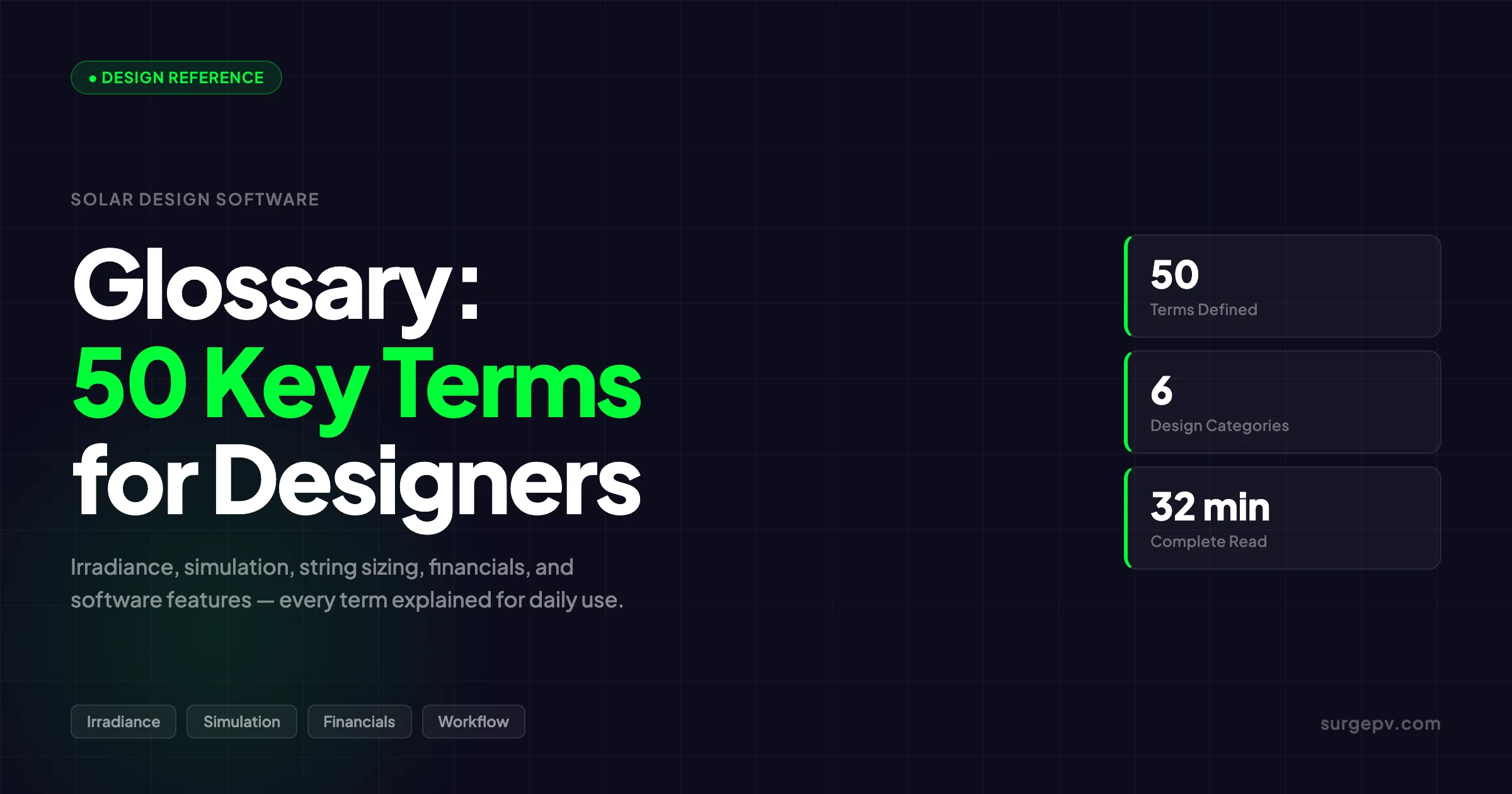
The vocabulary of solar PV design is not standardized across the industry. This glossary covers 50 terms that appear directly inside solar design software — from irradiance inputs and simulation outputs to electrical design parameters, financial metrics, and workflow features. Typical annual values: 900–1,100 kWh/m²/year in northern Europe; 1,600–2,200 kWh/m²/year in MENA and southern Europe. ### 2.
Every solar designer has encountered a colleague or client who uses a term differently — or a software field that’s labeled one way in one tool and another way elsewhere. The vocabulary of solar PV design is not standardized across the industry. One platform calls it “inverter loading ratio,” another calls it “DC:AC ratio,” and both mean exactly the same thing.
The vocabulary of solar PV design is not standardized across the industry. This glossary covers 50 terms that appear directly inside solar design software — from irradiance inputs and simulation outputs to electrical design parameters, financial metrics, and workflow features.
This glossary covers 50 terms that appear directly inside solar design software — from irradiance inputs and simulation outputs to electrical design parameters, financial metrics, and workflow features. Each definition is written for designers using software day-to-day, not for homeowners researching their first system. The focus is on what each term controls, how software uses it, and what happens to your design if you get it wrong.
TL;DR — What This Glossary Covers
50 solar design terms organized across 6 categories: solar resource and irradiance, module and component specifications, system design and configuration, simulation and performance metrics, financial and business terms, and software features. Each definition includes the practical implication for software-based design.
In this glossary:
- Solar resource and irradiance terms (GHI, DNI, POA, TMY, and more)
- Module specification terms that affect simulation accuracy
- System design parameters — DC:AC ratio, string sizing, voltage limits
- Simulation outputs — performance ratio, specific yield, P50/P90
- Financial model inputs — LCOE, NPV, PPA, MACRS
- Software workflow features — LiDAR, auto-stringing, BOM, SLD
Category 1: Solar Resource and Irradiance
These terms define the solar energy input to any simulation. If your irradiance data is wrong, everything downstream is wrong — yield estimates, financial models, and sizing calculations all inherit the error.
1. Global Horizontal Irradiance (GHI)
GHI is the total solar radiation received on a horizontal flat surface, measured in W/m² (instantaneous) or kWh/m² (cumulative over a period). It is the most commonly cited solar resource metric in weather datasets. For Global-specific compliance details, see Global net-metering-by-country. For Global-specific compliance details, see Global solar-permitting-speed-by-country.
Solar design software uses GHI as the primary input when the panel array is tilted. The software then decomposes GHI into its beam and diffuse components and recalculates the irradiance on your tilted array surface. You will not directly enter GHI — the software reads it from a weather dataset. What matters is choosing a high-quality dataset (NASA POWER, Meteonorm, Solargis, or PVGIS) whose GHI data is validated against ground measurements for your region.
Typical annual values: 900–1,100 kWh/m²/year in northern Europe; 1,600–2,200 kWh/m²/year in MENA and southern Europe. Also see: European Solar Incentives.
2. Direct Normal Irradiance (DNI)
DNI is the solar radiation received on a surface held perpendicular to the direction of the sun at any given moment. It measures only the beam component of sunlight — no diffuse sky radiation.
For standard flat-panel rooftop and ground-mount designs, DNI is used internally by the software’s transposition model, not entered directly by the designer. It becomes an explicit input for concentrated solar power (CSP) systems and dual-axis trackers where maximizing direct beam collection is the design objective. In flat-panel design, DNI data quality mainly affects performance ratio accuracy in high-DNI climates like the UAE or southern Spain. Also see: Spain net metering.
3. Diffuse Horizontal Irradiance (DHI)
DHI is the portion of solar radiation that has been scattered by the atmosphere and arrives from all directions of the sky dome rather than directly from the sun’s disc.
DHI is particularly important for systems in high-latitude or frequently overcast climates (UK, Germany, Netherlands) where diffuse radiation can represent 40–60% of annual GHI. East-west split arrays benefit disproportionately from high DHI environments because diffuse radiation is direction-independent. Software that only uses beam irradiance without accurate DHI data will underestimate production in cloudy climates. Also see: Germany solar subsidies. Read more about Battery Solar System Design UK.
4. Plane of Array (POA) Irradiance
POA irradiance is the actual irradiance hitting the surface of your solar panels — calculated by transposing horizontal irradiance data to match your array’s specific tilt and azimuth. It is the irradiance value that directly drives energy yield simulation.
This is the figure you should reference when reviewing simulation outputs. A common mistake is citing GHI from the weather dataset rather than POA in energy yield reports. For a 30° south-facing array at 48°N latitude, POA irradiance is typically 10–15% higher than GHI due to the favorable tilt geometry. Solar design software calculates POA automatically from GHI + DNI + DHI using transposition models like Perez or Hay-Davies.
5. Peak Sun Hours (PSH)
Peak Sun Hours is the number of hours per day (or year) during which solar irradiance averages 1,000 W/m² — the equivalent of full standard test conditions. A location with 5.0 PSH/day will produce the same total daily irradiance energy as 5 hours at exactly 1,000 W/m².
Software uses annual PSH to give designers a quick intuition for system sizing. A 10 kWp system at a site with 5.0 PSH/day will produce roughly 5.0 × 10 = 50 kWh/day before losses. PSH is also used in quick-sizing calculators before a full simulation run. It should not replace a full 8760-hour simulation for final design output.
6. Typical Meteorological Year (TMY)
A TMY dataset is a synthetic 8,760-hour weather file assembled from long-term historical data (typically 10–20 years) to represent a “typical” year rather than an exceptionally good or bad one. It contains hourly values for GHI, DNI, DHI, temperature, humidity, and wind speed.
Software uses TMY data as the irradiance backbone of every hourly simulation. The dataset source matters enormously — PVGIS satellite data is well-validated for Europe; Meteonorm interpolated data performs well for areas without ground measurement stations. When two simulations for the same site give different results, a different TMY source is almost always the explanation. Always note which TMY source is used in energy yield reports for projects requiring third-party validation.
7. Albedo
Albedo is the fraction of solar radiation reflected by the ground surface below and around the array, expressed as a value between 0 (no reflection) and 1 (total reflection). Standard software default is 0.2 (grass or typical ground).
Albedo significantly affects the rear-side irradiance of bifacial panels and becomes a critical input for any bifacial simulation. White roofing membranes have albedo values of 0.65–0.80. Snow cover reaches 0.75–0.90. Gravel has albedo of 0.15–0.25. For ground-mount bifacial systems, underestimating albedo by 0.2 can produce a 3–6% error in bifacial gain. Check the default in your software and adjust for the actual site surface. Read Bifacial Solar Panel Design Guide for a complete walkthrough.
8. Soiling Loss
Soiling loss is the reduction in energy output caused by dust, pollen, bird droppings, or other particulate matter accumulating on panel surfaces. It is expressed as a percentage of annual yield lost.
Most software applies a fixed annual soiling loss factor (default is often 2%). In reality, soiling loss is highly location-dependent — less than 0.5% per year in rainy northern Europe, up to 3–6% per year in dusty arid environments without regular cleaning. For utility-scale or commercial projects, use regional soiling data from Solargis or site-specific measurements. Soiling loss compounds with degradation over time, so a 3% soiling loss on a 15-year-old system means compounding losses are often underestimated.
Category 2: Module and Component Specifications
These terms appear directly in the component library of any design tool. Misreading them — or accepting software defaults without verification — introduces systematic errors into every simulation.
9. Standard Test Conditions (STC)
STC is the laboratory condition under which solar panels are rated: 1,000 W/m² irradiance, 25°C cell temperature, and an air mass of 1.5. Every panel’s rated power (e.g., 420 Wp) is measured at STC.
Real-world conditions rarely match STC — irradiance fluctuates, and operating cell temperatures typically reach 45–65°C in summer. Software converts STC-rated power to real-world output using temperature coefficient adjustments and irradiance corrections. This means a 420 Wp panel operating at 55°C cell temperature and 900 W/m² irradiance might only deliver 375 W at that moment. Always use STC ratings for component selection, but rely on simulated output (not nameplate power) for yield estimates.
10. Nominal Operating Cell Temperature (NOCT)
NOCT is the cell temperature a module reaches under defined “open-rack” outdoor conditions: 800 W/m² irradiance, 20°C ambient air, and 1 m/s wind speed. Published on every panel datasheet.
Software uses NOCT — along with the ambient temperature time series from the TMY dataset — to estimate operating cell temperature at each simulation timestep. The formula is: T_cell = T_ambient + (NOCT − 20°C) / 800 × G, where G is irradiance. NOCT values typically range from 42–49°C. Lower NOCT means lower operating temperature and higher real-world output. When comparing panels of identical rated power, a lower NOCT panel will outperform in hot climates.
11. Temperature Coefficient (Pmax)
The temperature coefficient of maximum power (Pmax) describes how much a panel’s power output changes with temperature, expressed as %/°C. Standard monocrystalline silicon panels have a Pmax temperature coefficient of approximately −0.35 to −0.45%/°C.
This means for every degree Celsius above 25°C (STC reference), the panel loses 0.35–0.45% of its rated output. At 65°C operating cell temperature — common on hot summer days — a panel with −0.40%/°C loses 16% of its rated power. TOPCon and HJT cells have lower temperature coefficients (−0.25 to −0.30%/°C) and perform meaningfully better in hot climates. Accurate simulation requires the software to apply this coefficient to every hour of the TMY temperature profile.
12. Annual Degradation Rate
The annual degradation rate is the percentage by which a solar panel’s output declines per year due to light-induced degradation, material aging, and UV exposure. The industry standard is 0.5–0.7% per year for quality monocrystalline modules.
Over a 25-year lifetime, a panel degrading at 0.5%/year retains approximately 88% of its original output at year 25 (using the compounding formula). Most software applies a linear degradation model. When comparing panel options, check the warranty degradation guarantee — some premium manufacturers guarantee 0.25–0.30%/year degradation, which adds measurable lifetime yield over 25 years. A 1% reduction in annual degradation rate on a 500 kWp commercial system can be worth €15,000–25,000 in lifetime revenue.
13. Bifacial Gain
Bifacial gain is the additional energy production a bifacial panel achieves from rear-side light collection, expressed as a percentage of front-side output. Typical bifacial gains are 5–15% depending on mounting height, row spacing, and ground albedo.
Software simulates bifacial gain using the bifaciality factor of the module (typically 0.70–0.80) combined with the rear-side irradiance calculation, which depends on albedo, mounting height, and row-to-row shading geometry. For flat commercial rooftops with white membranes (albedo 0.65–0.75), bifacial gain often reaches 8–12%. For systems at 300mm roof clearance over dark membranes, it may be only 2–4%. Never accept the default bifacial gain in software without verifying the albedo input and mounting geometry. Shadow analysis software identifies shading issues before installation.
14. Fill Factor
Fill Factor (FF) is the ratio of a panel’s actual maximum power output to the product of its open-circuit voltage and short-circuit current. It measures how “square” the IV curve is. Commercial monocrystalline panels have fill factors of 0.78–0.84.
Higher fill factor indicates a panel with lower internal resistance and better performance at the actual operating point. Software uses fill factor implicitly when modeling the IV curve — it affects how well the MPPT algorithm captures available power under non-uniform shading or partial cloud cover. Fill factor also declines as panels age. When simulating long-term performance, software that models IV curve degradation (not just power degradation) produces more accurate multi-decade yield projections.
15. IV Curve
The IV curve is a graph plotting the current output of a solar panel against its voltage at every operating point from short circuit (Isc at V=0) to open circuit (Voc at I=0). The knee of the curve is the Maximum Power Point (MPP).
Software uses IV curve data to model how panels behave when partially shaded (leading to partial IV curves), how mismatched strings interact (combining IV curves), and how MPPT inverters seek the optimal operating point. Understanding the IV curve shape is necessary when diagnosing why a simulated performance ratio is lower than expected, or when evaluating whether bypass diodes are mitigating shade losses effectively.
16. Open Circuit Voltage (Voc)
Voc is the maximum voltage a solar panel produces when no current is flowing — under full irradiance with the output circuit open. It is the highest voltage a string of panels can reach.
String Voc at the lowest expected temperature determines whether the string exceeds the inverter’s maximum input voltage rating — a critical safety and compliance check. Voc increases as temperature falls. At −10°C, a string of 20 panels with Voc of 41.0 V each will reach approximately 880–920 V depending on the temperature coefficient, which may exceed the 1,000 V limit of many residential inverters. Solar design software runs this check automatically for the minimum temperature in the TMY dataset.
17. Short Circuit Current (Isc)
Isc is the current that flows from a solar panel when its output terminals are directly connected (short-circuited) with zero resistance. It represents the maximum current the panel can produce under given irradiance conditions.
Software uses Isc to verify that string current stays within the inverter’s maximum DC input current per MPPT channel, and to size overcurrent protection devices (fuses, breakers) correctly. For parallel string configurations, Isc from multiple strings adds up. A combiner box feeding six parallel strings of panels with Isc = 12.0 A each has a worst-case backfeed current of 60 A that the overcurrent protection must handle.
Category 3: System Design and Configuration
These are the parameters you set directly in the design tool. Each one has a right range — and operating outside it either violates code, damages equipment, or leaves production on the table.
18. DC:AC Ratio (Inverter Loading Ratio)
The DC:AC ratio — also called the Inverter Loading Ratio (ILR) — is the total installed DC module capacity (in kWp) divided by the inverter’s rated AC output capacity (in kW). A 10 kWp array connected to an 8 kW inverter has a DC:AC ratio of 1.25.
Industry-standard range is 1.1–1.35. Lower ratios (closer to 1.0) waste inverter capacity and increase cost per kWh. Higher ratios (above 1.4) increase inverter clipping losses, voiding the economic benefit of the oversized array. Solar design software calculates expected clipping loss for any ratio so you can find the optimal balance for each project’s irradiance profile and electricity tariff structure. For sites with time-of-use rates that reward morning or evening generation, a lower DC:AC ratio with less clipping may be more valuable than a higher ratio optimized for peak production.
19. MPPT (Maximum Power Point Tracking)
MPPT is the algorithm an inverter uses to continuously adjust its operating voltage to keep each string of panels at the voltage where they produce maximum power. The maximum power point changes with irradiance, temperature, and shading conditions.
The number of MPPT inputs on an inverter is a key design parameter in software. Each MPPT channel handles one independent string or group of strings with the same orientation and shading profile. A building with panels on a south face, an east face, and a west face requires at least 3 MPPT inputs — one per orientation — to prevent higher-producing strings from pulling lower-producing strings away from their respective optimal operating points. Mismatching orientations on a single MPPT channel is one of the most common design errors, and software that enforces MPPT separation catches it before installation.
20. String Configuration
String configuration defines how many solar panels are connected in series (a string) and how many strings are connected in parallel before entering an inverter MPPT input. Series connections increase voltage; parallel connections increase current.
Software calculates the valid string range automatically: minimum strings to maintain voltage above the inverter’s minimum MPPT voltage at maximum temperature, maximum strings to keep Voc below the inverter’s maximum input voltage at minimum temperature. Strings outside this range either fail to operate or damage the inverter. The optimal string length within the valid range is usually determined by roof geometry (fitting whole strings without cutting panels) and desired current per MPPT.
21. Azimuth
Azimuth is the compass direction a solar array faces, measured in degrees clockwise from true north. South-facing panels in the northern hemisphere have an azimuth of 180°.
In software, azimuth is entered for each roof surface or module group. True south (180°) produces maximum annual yield. Deviations of ±15° from south reduce annual output by approximately 1–3%. Deviations of ±45° reduce output by 5–8%. East-west split arrays (90° and 270°) each produce 20–25% less than a south array at the same tilt but provide a flatter daily generation profile, which improves self-consumption for sites with morning and afternoon loads. Software models azimuth-dependent yield differences and can compare multiple layout orientations automatically.
22. Tilt Angle
Tilt angle is the angle of the panel surface from horizontal. A panel lying flat on the ground has a tilt of 0°; a panel mounted vertically has a tilt of 90°.
The optimal tilt for annual energy yield approximates the site latitude. At 48°N (central Europe), the optimal tilt is roughly 30–35°. At 25°N (Middle East), it is closer to 15–20°. Software calculates annual POA irradiance at any tilt-azimuth combination using the TMY dataset. For flat commercial rooftops, software helps designers balance yield improvement from higher tilt against inter-row shading losses and structural wind load constraints. Ballasted racking on flat rooftops typically uses 5–15° tilt as a compromise.
23. Inverter Clipping
Inverter clipping occurs when the DC power produced by panels exceeds the inverter’s maximum AC output capacity. The inverter limits its output and the surplus DC power is wasted.
Clipping is acceptable in controlled amounts — typically 0.5–3% of annual production for a well-sized system. Software calculates clipping loss as part of the loss waterfall, usually displayed in the simulation output. Clipping only occurs on the highest irradiance hours (peak summer midday), and the panels producing excess power shift their operating point down the IV curve to reduce current. The economic cost of clipping should be weighed against the savings from using a smaller inverter and the benefit of capturing early-morning and late-evening production when irradiance is below clipping threshold.
24. Voltage Drop
Voltage drop is the reduction in voltage that occurs as current flows through resistance in cables between the array, inverter, and AC connection point. Excessive voltage drop wastes energy as heat in the wiring.
IEC 62109 and NEC 690 both recommend keeping DC voltage drop below 1–2% per segment (string to combiner, combiner to inverter). Software calculates voltage drop for any cable size, length, and current combination using Ohm’s law. The relevant formula: V_drop = 2 × L × I × ρ / A, where L is one-way cable length, I is current, ρ is copper resistivity (1.72 × 10⁻⁸ Ω·m), and A is cable cross-section in m². For detailed cable sizing guidance, the solar cable sizing calculation post covers the full methodology.
25. Overcurrent Protection Device (OCPD)
An Overcurrent Protection Device (OCPD) is a fuse or circuit breaker installed to protect wiring and components from short-circuit and overcurrent damage. In PV systems, string fuses and DC disconnect breakers are the primary OCPDs.
Software generates the overcurrent protection values required for each segment of the system. For string fuses in parallel configurations, the minimum fuse rating must exceed the string Isc; the maximum rating must not exceed the module’s maximum series fuse rating listed on the datasheet. Getting this wrong causes either nuisance tripping (fuse too small) or unchecked fault current that damages modules (fuse too large). Permit packages generated by software include OCPD specifications for each string and combiner.
26. Rapid Shutdown
Rapid shutdown (NEC 690.12) is a code requirement mandating that PV system voltage and current in roof conductors be reduced to safe levels within 30 seconds of initiating shutdown. Required on all roof-mounted systems in NEC 2023 jurisdictions regardless of building height.
From a software perspective, rapid shutdown compliance affects component selection. Systems must use module-level power electronics (MLPEs — microinverters or power optimizers) or listed rapid shutdown devices to comply. Software that integrates NEC compliance checks will flag designs using standard string configurations on rooftops in NEC 2023 jurisdictions. This constraint directly affects the inverter and module choices available in the component library.
Category 4: Simulation and Performance Metrics
These are the outputs that determine whether your design is good. Understanding what each number means — and what drives it — is the difference between using software as a black box and using it as a real design tool.
27. Specific Yield
Specific yield is total annual energy production (kWh) divided by installed DC capacity (kWp), giving kWh/kWp/year. It is the most useful metric for comparing designs across different system sizes at the same site.
A 10 kWp system producing 11,000 kWh/year has the same specific yield (1,100 kWh/kWp) as a 100 kWp system producing 110,000 kWh/year. The larger number tells you nothing about design quality; the specific yield does. Typical values: 850–1,100 kWh/kWp in northern Europe, 1,200–1,600 kWh/kWp in southern Europe, 1,600–2,000 kWh/kWp in MENA. When comparing two layout options for the same roof, the one with higher specific yield is the better-performing design.
28. Performance Ratio (PR)
Performance Ratio is the ratio of actual annual energy output to the energy the system would produce if it operated at STC efficiency for every hour of available irradiance. It is expressed as a percentage and accounts for all real-world losses.
PR = Actual yield (kWh) / (POA irradiance (kWh/m²) × Module area (m²) × Module STC efficiency)
Well-designed systems achieve PR values of 75–85%. Below 70% suggests significant design inefficiencies or losses. Above 85% is possible in cold northern climates where low temperatures improve output. Software breaks down the PR into individual loss contributions so you can identify which loss category (temperature, shading, wiring, or inverter) is the main drag. See the full performance ratio glossary entry for detailed calculation methodology.
29. Capacity Factor
Capacity Factor is the ratio of a system’s actual annual energy output to its theoretical maximum if it operated at full rated power for every hour of the year (8,760 hours). It is expressed as a percentage.
For solar PV, typical capacity factors are 10–20%. A system in southern Spain might reach 20–22%; a system in Scotland might be 10–12%. Software calculates capacity factor automatically from simulation results. It is primarily used in utility-scale project analysis and investment screening. For residential and commercial projects, specific yield and performance ratio are more actionable metrics because they directly describe design quality rather than site resource.
30. P50 / P90 Energy Yield
P50/P90 values describe the probability distribution of annual energy yield across many possible weather years. P50 is the median — the system is equally likely to produce above or below this figure. P90 is the yield expected to be met or exceeded in 9 out of 10 years.
Lenders financing solar projects require P90 figures to protect against downside risk. P90 is typically 5–10% below P50 for rooftop systems and 8–15% below for utility-scale projects where modeling uncertainty is higher. Software generates P50 and P90 by applying statistical uncertainty factors to the base TMY simulation. When presenting yield estimates to investors or financiers, always specify whether you are quoting P50 or P90.
31. Loss Analysis (Loss Waterfall)
The loss analysis (or loss waterfall) is a breakdown of all the factors that reduce a solar system’s output from theoretical maximum (100% of module STC rating × irradiance) to actual yield. It quantifies each loss category as a percentage.
Typical loss categories in software: irradiance losses (shading, horizon, reflectance, IAM), DC losses (temperature, wiring, module mismatch, degradation, soiling), inverter losses (conversion efficiency, clipping), and AC losses (transformer, cable). A complete loss analysis lets you identify where the biggest gains are available. If shading losses are 8% but temperature losses are only 3%, redesigning the layout to reduce shading delivers more value than switching to lower temperature coefficient panels.
32. 8760-Hour Simulation
An 8760-hour simulation (or hourly simulation) models system performance at every hour of the year (8,760 hours = 365 days × 24 hours), using the TMY weather dataset as input for each timestep.
This is the industry standard for yield estimation and is required by most financiers and technical due diligence processes. It produces a full hourly time series of power output, which software uses to model battery dispatch, demand charge analysis, and self-consumption calculations. Simpler tools use monthly irradiance averages rather than hourly data — these are useful for quick estimates but can be 5–15% off on systems with complex shading patterns or time-of-use tariff optimization requirements.
33. Anti-Islanding
Anti-islanding is the automatic shut-down behavior of a grid-tied inverter when it detects that the utility grid has gone offline. The inverter stops exporting power to prevent energizing a section of grid that utility workers might believe is de-energized.
Anti-islanding protection is mandatory in virtually all markets for grid-tied systems. From a software perspective, the relevant check is ensuring the inverter’s listed anti-islanding method (passive frequency detection, active frequency shifting, or grid impedance measurement) meets the local grid code requirement (IEEE 1547, VDE-AR-N 4105, G99, AS 4777, etc.). Software that includes grid code compliance checks flags inverter selections that lack the required anti-islanding certification for the project market.
34. Total Solar Resource Fraction (TSRF)
TSRF is a metric that combines tilt, azimuth, and shading effects into a single percentage representing how much of the site’s maximum possible solar resource reaches a specific roof area. A south-facing 30° roof with no shading in a given location has a TSRF of 100%.
Software calculates TSRF for each module placement position. It is a useful metric for quickly assessing whether a specific roof section is worth installing on. Roof areas with TSRF below 60% typically produce insufficient yield to justify installation cost. TSRF also serves as a quick communication tool with clients — it conveys “this section of your roof captures 85% of the available solar resource” without requiring clients to understand irradiance mathematics.
35. Soiling Degradation Modeling
Soiling degradation modeling is the simulation of how accumulated soiling loss changes over time based on local precipitation frequency, particulate matter concentration, and cleaning schedules. It is a more sophisticated version of the fixed soiling loss factor.
Advanced software applies monthly soiling factors based on rainfall data — high soiling loss in dry summer months, lower loss during wet winters. For commercial and utility projects where O&M planning drives ROI, soiling modeling informs optimal cleaning frequency. A site with 4% soiling loss in August but cleaning scheduled only annually might benefit from bi-annual cleaning that recovers 1.5–2% of annual production. The generation and financial tool includes soiling scenarios in multi-year cashflow projections.
Category 5: Financial and Business Terms
Solar design software increasingly includes financial modeling alongside yield simulation. These terms define the economic outputs that clients and investors actually make decisions from.
36. LCOE (Levelized Cost of Energy)
LCOE is the total lifetime cost of a solar system (installation, financing, O&M, decommissioning) divided by the total lifetime energy output, giving a cost per kWh. It is the standard metric for comparing solar against other energy sources and against the local grid tariff.
LCOE formula: (Total Upfront Cost + Discounted O&M Costs) / (Annual kWh × Σ(1/(1+r)^n) for n years), where r is the discount rate. Software calculates LCOE automatically when you enter system cost, O&M assumptions, and discount rate. In 2025–2026, utility-scale solar LCOE in southern Europe reached €20–35/MWh, below gas peaking at €80–120/MWh. For residential systems, LCOE of €55–90/MWh typically undercuts retail electricity tariffs.
37. Payback Period
Payback period is the number of years required for cumulative energy savings to equal the initial investment. It is the simplest financial metric and the one most clients ask about first.
Simple payback = System cost (€) / Annual savings (€/year). For a €12,000 system saving €1,800/year, simple payback = 6.7 years. Software calculates both simple payback and discounted payback (which accounts for the time value of money). Discounted payback is always longer than simple payback. For an honest client conversation, quote simple payback as the headline and show discounted payback in the supporting financial model.
38. Net Present Value (NPV)
NPV is the sum of all future project cashflows discounted back to today’s money, minus the initial investment. A positive NPV means the project creates economic value over its lifetime.
NPV = Σ(Annual savings / (1 + discount rate)^year) − Initial investment. For a 25-year residential solar system, NPV is highly sensitive to the discount rate assumption and electricity price escalation rate. A 5% discount rate versus 8% can change NPV by 20–30% on the same project. Software should let you test multiple discount rate and electricity escalation scenarios. If the NPV is only positive under optimistic assumptions, be transparent about the sensitivity.
39. MACRS Depreciation
MACRS (Modified Accelerated Cost Recovery System) is the US federal tax depreciation schedule for solar assets. Commercial solar systems qualify for 5-year MACRS, allowing accelerated depreciation that substantially improves after-tax ROI.
Under MACRS, approximately 40% of the installed cost can be depreciated in year 1 (using the 200% declining balance method), with remaining value spread across years 2–6. Combined with the Investment Tax Credit (ITC), MACRS can recover 50–60% of the installed cost in tax benefits within the first two years for qualifying commercial projects. Software that models US commercial solar should include MACRS alongside ITC in after-tax cashflow projections. Ignoring depreciation produces significantly conservative ROI estimates.
40. Power Purchase Agreement (PPA)
A Power Purchase Agreement is a long-term electricity sales contract in which a solar developer sells power to a customer (or utility) at an agreed price per kWh for the contract duration, typically 15–25 years. The developer owns, operates, and maintains the system.
From a software perspective, PPAs require modeling the annual kWh output for every contract year (incorporating degradation), the escalated PPA rate over the contract term, and the residual value at contract end. Software needs to produce a bankable yield report for each year of the contract to satisfy financier requirements. PPA pricing is set as a discount to the expected future grid tariff — solar yield simulation accuracy directly determines whether the PPA is profitable.
41. Escalator Rate
The escalator rate (or electricity price escalation rate) is the assumed annual percentage increase in retail electricity tariffs used in financial models. It determines the growing value of solar-generated electricity over the system’s lifetime.
A 3% annual escalator means electricity that costs €0.30/kWh today will cost €0.49/kWh in 20 years. Small changes in the escalator rate produce large differences in 25-year NPV. For European residential models, using 2–4% escalation is well-supported by historical data. For commercial projects, using the regulator’s published long-run marginal cost forecast or the specific utility’s rate increase history is more defensible. Never use a single escalator rate without showing the client how NPV changes across a 1–5% escalator range.
42. Demand Charge
A demand charge is a component of commercial utility billing based on the peak power demand (kW) drawn during the billing period, rather than on total energy consumed (kWh). Demand charges can represent 30–60% of a commercial electricity bill.
Solar alone rarely eliminates demand charges — a single cloudy morning with full load can set the monthly peak before the panels generate anything. Software that models demand charges must simulate power demand and solar generation at 15-minute intervals to identify whether the peak draw occurs at times when solar production reduces demand. Battery storage paired with solar is often the effective solution for demand charge reduction. The generation and financial tool models demand charge savings with and without storage. See Adding Battery Storage Services for detailed guidance.
43. Yield Ratio (kWh/kWp)
The yield ratio is the specific yield of the system — annual energy output in kWh divided by installed capacity in kWp. It is mathematically identical to specific yield but is used explicitly in financial models to convert from system size to projected annual revenue.
Annual revenue = System size (kWp) × Yield ratio (kWh/kWp) × Electricity price (€/kWh). For a 200 kWp commercial system in Munich (yield ratio ~1,000 kWh/kWp) with electricity at €0.22/kWh: Annual savings ≈ 200 × 1,000 × €0.22 = €44,000/year. The yield ratio is the single number that connects the technical simulation to the financial model, which is why simulation accuracy directly determines the quality of client proposals.
Category 6: Software Features and Workflow
These terms describe the tools inside design platforms — features that automate work that used to require hours of manual calculation or separate software packages.
44. LiDAR Roof Modeling
LiDAR (Light Detection and Ranging) roof modeling uses point cloud data from aerial LiDAR surveys to create a precise 3D model of a roof — including ridge lines, valley lines, pitch angles, obstructions (HVAC units, vents, skylights), and exact surface dimensions.
LiDAR-based designs require fewer or no site visits, produce more accurate panel counts, and enable precise shading analysis from roof obstructions. For large commercial rooftops, a LiDAR-sourced roof model reduces measurement error from ±5% (tape measure) to ±0.3% (LiDAR). Software that integrates national LiDAR datasets (available for most of the UK, Netherlands, Germany, and US urban areas) can generate roof models automatically from the address without manual input. This is one of the fastest-moving capability areas in solar design software. See our guide on Community Solar Projects Germany for more.
45. Auto-Stringing
Auto-stringing is a software feature that automatically calculates the optimal string configuration — panels per string, number of parallel strings, inverter MPPT allocation — based on the components selected, site conditions, and applicable electrical code limits.
Manual string sizing requires checking Voc at minimum temperature, Vmp at maximum temperature, and current limits for each MPPT channel separately. For a complex commercial system with multiple roof faces and mixed orientations, this can involve dozens of configuration checks. Auto-stringing runs every valid configuration automatically, flags non-compliant options, and ranks compliant options by yield or cost. Reviewing the auto-stringing output (rather than accepting it blindly) is still necessary — software does not always know which faces belong to the same roof segment or share a common combiner.
46. Bill of Materials (BOM)
A Bill of Materials is the complete list of every component required to install a solar system — modules, inverters, mounting hardware, cables, combiners, disconnect switches, meters, monitoring equipment, and balance-of-system items — with quantities and specifications for each.
Software generates BOMs automatically from the design file, which eliminates the manual counting and transcription errors that plague spreadsheet-based BOMs. An accurate BOM is the foundation of accurate cost estimation and procurement. For installers quoting multiple projects per week, auto-generated BOMs represent several hours of time savings per project. BOMs exported from solar design platform can feed directly into procurement systems and ERP platforms through CSV or API integrations.
47. Single-Line Diagram (SLD)
A Single-Line Diagram (SLD), also called a one-line diagram, is a simplified electrical schematic showing the flow of power through the system using single lines to represent multi-conductor cables. It shows all major components, protection devices, disconnects, and interconnection points.
The SLD is a core document in the permit package. AHJs (Authorities Having Jurisdiction) require it for building permit applications, and utilities require it for interconnection applications. Software auto-generates SLDs from the design file, including the correct OCPD ratings, cable sizes, and equipment specifications. Auto-generated SLDs eliminate the drafting step that used to require a separate CAD tool or manual Visio diagram for each project.
48. Permit Package (Plan Set)
A permit package (or plan set) is the complete set of engineering drawings and documentation submitted to the local AHJ to obtain a building and electrical permit for a solar installation. It typically includes the site plan, roof plan with panel layout, SLD, elevation drawings, structural calculations, and equipment cut sheets.
Software that generates permit packages automatically reduces the per-project permit preparation time from 2–4 hours to 15–30 minutes. Package formats must match AHJ-specific requirements — some jurisdictions accept digital submissions with standardized layouts; others have custom title block and checklist requirements. For installers operating across multiple jurisdictions, software with a library of AHJ-specific templates is significantly more efficient than manually adjusting a standard package. See the permit package generation glossary entry for format details.
49. Shade Report
A shade report is a document quantifying the shading losses at a specific site — typically including a 3D visualization of the roof with color-coded irradiance mapping, monthly and annual shading loss percentages, and a sun path diagram showing when and where shading occurs.
Shade reports serve two purposes: technical (informing panel placement and stringing decisions) and commercial (showing clients exactly why certain roof sections are excluded or deprioritized). Software generates shade reports from 3D site models, using horizon profiles from digital elevation data and near-shade modeling from the 3D roof model with obstructions. A shade report with a 15% annual shading loss on a proposed section is a clear basis for repositioning panels to a lower-shading area. For a deeper dive on analysis tools, see solar shading analysis tools.
50. Proposal Generation
Proposal generation in solar design software refers to the automated creation of client-facing sales proposals directly from the design file — including system specifications, yield estimates, financial analysis, company branding, and product imagery — without manual data transfer or reformatting.
The quality gap between software-generated proposals and manually assembled PDFs is significant. A software-generated proposal pulls the exact simulation results, financials, and component specifications from the design into a pre-structured branded document in minutes. Manual proposals require re-entering data, reformatting tables, and updating figures across multiple sections. Data entry errors in manual proposals — wrong system size, wrong annual production, wrong payback period — are common and damage client trust. The solar proposal software built into SurgePV generates proposals directly from completed designs, including interactive elements for client self-serve financing comparisons. Read more about Agricultural Solar Case Study.
Design Smarter With Every Term in Practice
SurgePV’s solar design platform gives you LiDAR modeling, auto-stringing, 8760-hour simulation, and proposal generation in a single workflow — no manual data re-entry between tools.
Book a DemoNo commitment required · 20 minutes · Live project walkthrough
For a direct comparison, see Arka 360 vs SurgePV.
How These Terms Work Together in a Real Design
Understanding terms in isolation is useful. Understanding how they connect in a real software workflow is where the knowledge becomes actionable.
A typical design workflow in cloud solar design tool flows like this:
-
Site resource input: The software loads a TMY dataset for the site location, providing hourly GHI, DNI, and DHI values across 8,760 hours.
-
Array configuration: You define tilt, azimuth, string configuration, and DC:AC ratio. The software validates Voc at minimum temperature and flags any string lengths outside the inverter’s input range.
-
Shading analysis: Using the 3D roof model (LiDAR or satellite-derived), the software calculates near shading and horizon shading losses for each module position, producing the shade report and TSRF values.
-
Simulation: The 8760-hour engine calculates hourly POA irradiance at each module position, applies temperature coefficients, soiling factors, degradation, wiring losses, and inverter efficiency curves to produce the annual yield, specific yield, and performance ratio.
-
Loss waterfall: The simulation outputs a loss analysis showing every contribution to the gap between STC nameplate power and actual yield.
-
Financial model: Annual yield feeds into the financial tool, which applies electricity tariff data, escalation rates, MACRS depreciation, and ITC to produce payback period, NPV, LCOE, and P50/P90 figures.
-
Document generation: The design file auto-generates the SLD, permit package, BOM, shade report, and client proposal — all using the same verified data from step 3 onward.
Pro Tip — Use Specific Yield to Spot Errors
Before reviewing any other simulation output, check the specific yield against the regional benchmark. If your simulation shows 700 kWh/kWp in Madrid or 1,500 kWh/kWp in Oslo, something is wrong — either the irradiance dataset is not loading correctly or a loss factor is misconfigured. Specific yield is the fastest sanity check in any simulation.
Where to Go From Here
The 50 terms in this glossary cover the full vocabulary of solar design software — from the irradiance inputs that start every simulation to the proposals that close sales. You do not need to memorize every formula, but you do need to understand what each term controls and what changes if you get it wrong.
For deeper coverage of individual terms, SurgePV’s glossary has detailed articles on most of the terms referenced here. For applied design methodology — how these concepts come together in a real system design process — the solar design principles guide covers the full engineering workflow from site assessment to commissioning.
Three things to take away:
- Always verify the TMY irradiance source and input albedo before trusting any simulation output
- Specific yield and performance ratio are the two numbers that tell you whether a design is actually good
- Auto-generated BOMs, SLDs, and permit packages are only as accurate as the underlying design — verify the design, not just the documents
Frequently Asked Questions
What is the most important term to understand in solar design software?
Performance Ratio (PR) is arguably the single most important term because it measures how efficiently a real system converts available irradiance into usable electricity. A well-designed system using accurate solar design software should achieve a PR of 75–85%. If your simulated PR is outside that band, it usually signals an error in string sizing, shading losses, or system loss assumptions. Also see: Us Residential Solar Market Trends 2026.
What is the difference between GHI, DNI, and DHI in solar design software?
GHI (Global Horizontal Irradiance) is the total solar radiation on a horizontal surface. DNI (Direct Normal Irradiance) is the solar radiation received on a surface perpendicular to the sun’s rays — most relevant for concentrated solar and tracking systems. DHI (Diffuse Horizontal Irradiance) is scattered skylight that reaches a horizontal surface. Solar design software uses all three components to calculate the Plane of Array (POA) irradiance, which is the actual irradiance hitting your tilted panels.
What does DC:AC ratio mean in solar design?
The DC:AC ratio (also called inverter loading ratio or ILR) is the installed DC module capacity divided by the inverter’s AC output capacity. A ratio of 1.2 means you have 1.2 kWp of panels for every 1 kW of inverter capacity. The industry standard range is 1.1–1.35. Higher ratios reduce cost per kWh but increase clipping losses. Solar design software calculates clipping loss automatically so you can optimize the ratio for each project.
What is the difference between P50 and P90 in solar energy yield modeling?
P50 is the median energy yield — the amount the system is equally likely to exceed or fall short of. P90 is a conservative estimate that the system will meet or exceed in 90% of years. Lenders and investors typically require P90 yield figures for project financing. P90 is usually 5–10% lower than P50 for a typical rooftop system. Solar design software generates both values using multi-year irradiance datasets and uncertainty modeling.
How is performance ratio calculated in solar design software?
Performance Ratio = (Actual energy output in kWh) / (Irradiance on array in kWh/m² × Module area in m² × Module efficiency). In practice, solar design software calculates it by summing all system losses — temperature losses, wiring losses, soiling, shading, inverter efficiency, and availability — to arrive at the ratio of actual output to theoretical maximum. A PR of 80% means the system delivers 80% of what it would under ideal conditions.
What is specific yield and why does it matter for solar designers?
Specific yield is total annual energy output (kWh) divided by installed DC capacity (kWp), expressed in kWh/kWp/year. It strips out system size and lets you compare designs directly. A rooftop in Munich typically achieves 950–1,050 kWh/kWp/year, while the same design in Seville might reach 1,600–1,800 kWh/kWp/year. When you compare two system configurations for the same site, the one with higher specific yield is the better design.