Quick Answer
A 1 MW commercial solar array in California will not save a manufacturing plant from its demand charge bill. The utility bills the plant for 920 kW of demand at $22 per kW. The worked example tracks one real-shape 1.2 MW facility from interval data through a sized 600 kW / 1,200 kWh BESS plus 800 kW solar array.
A 1 MW commercial solar array in California will not save a manufacturing plant from its demand charge bill. Not on its own. The plant’s monthly peak demand event lands at 6:45 p.m. on a Tuesday in August, when the array is producing 80 kW into a clear sky and falling fast. The utility bills the plant for 920 kW of demand at $22 per kW. The solar saved the facility $0.50 on that bill.
A 1 MW commercial solar array in California will not save a manufacturing plant from its demand charge bill. The utility bills the plant for 920 kW of demand at $22 per kW. The worked example tracks one real-shape 1.2 MW facility from interval data through a sized 600 kW / 1,200 kWh BESS plus 800 kW solar array.
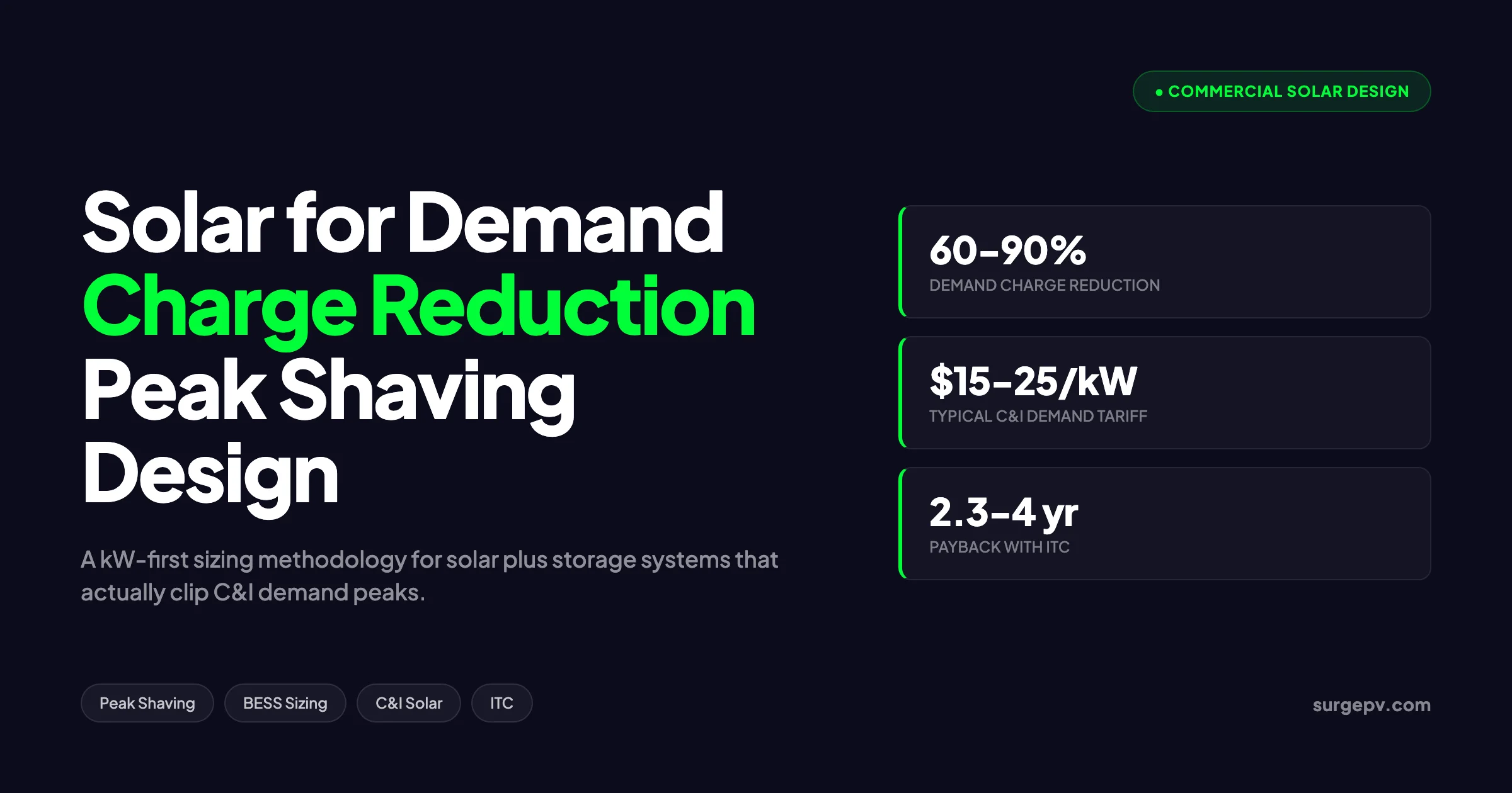
This is the design problem that drives almost every peak shaving project in commercial and industrial solar today. Demand charges represent 30 to 70 percent of a C&I electric bill in markets with meaningful capacity pricing — California, Massachusetts, New York, Illinois, parts of Texas — and a solar array sized only against energy consumption misses most of that revenue. The fix is a combined solar plus battery design where the PV cuts daytime peaks and the battery suppresses everything the sun cannot reach. Done well, the system pays back in 2.3 to 4 years. Done badly, the same hardware delivers half that.
This guide walks through the design discipline behind peak shaving for C&I solar: how demand charges actually price your peak, why solar alone usually fails to address them, the five-step kW-first sizing methodology that makes the system bankable, and the dispatch control logic that determines whether the battery actually clips the peak when it matters. Every number is sourced. The worked example tracks one real-shape 1.2 MW facility from interval data through a sized 600 kW / 1,200 kWh BESS plus 800 kW solar array.
TL;DR — Solar Demand Charge Reduction Design
Demand charges price your single highest 15-minute average power draw of the month, often at $15 to $25 per kW. Solar reduces them only when production overlaps the billing peak — which it usually does not. Combined solar plus storage, sized kW-first from interval data and controlled by a forecasting EMS, can cut C&I demand charges by 60 to 90 percent and deliver 2.3 to 4 year payback under the IRA Section 48E ITC. Standalone PV without storage typically achieves 10 to 30 percent demand charge reduction in C&I tariffs.
In this guide:
- How C&I demand charges are calculated, including ratchets and time-of-use demand windows
- Why solar alone rarely cuts demand charges below 30 percent in three-shift or evening-peak facilities
- The five-step kW-first sizing methodology for peak shaving solar plus BESS
- A fully worked example: 1.2 MW manufacturing plant → 800 kW PV + 600 kW / 1,200 kWh BESS
- Dispatch control strategies that determine whether the battery actually shaves the peak
- Common design mistakes — vendor-default cabinet sizing, ignoring ratchets, undersized inverters
- ROI math under the IRA 48E ITC, with sensitivity to demand charge tariff and event distribution
- When peak shaving is not the right strategy — facilities where load shifting or solar self-consumption dominate
How C&I Demand Charges Actually Price Your Peak
Demand charges are not energy charges. The utility meters two things every billing month: total kilowatt-hours consumed (the energy charge) and the highest 15-minute or 30-minute average power draw (the demand charge). The demand charge is then priced at a fixed dollar amount per kilowatt regardless of how briefly that peak event occurred.
A facility that runs at 200 kW steady all month and spikes to 500 kW for exactly 15 minutes on the third Tuesday will be billed for 500 kW of demand. The 200 kW baseline is irrelevant to the demand line item. The single highest interval sets the bill.
This pricing structure produces an asymmetric design problem. Peak shaving has to suppress one event per month — the worst one — and a system that handles the average event but misses the 99th percentile spike delivers near-zero demand charge savings. The tariff rewards perfection, not consistency.
Demand Charge Components in Modern C&I Tariffs
Most C&I tariffs in the United States layer two or three demand charges on the same bill: For United States-specific compliance details, see United States arizona/phoenix.
- Facility demand charge (non-coincident peak) — priced on the single highest 15- or 30-minute interval of the billing month, regardless of when it occurred. Typically $5 to $12 per kW.
- On-peak demand charge — priced on the highest interval that fell inside the utility’s defined on-peak window, often 12 p.m. to 8 p.m. on weekdays. Typically $10 to $25 per kW. This is the line item solar can address most directly.
- Generation or capacity demand charge — applied during the utility’s annual coincident peak hour, sometimes only known retroactively. PJM, ISO-NE, and NYISO territories include this. Typically $3 to $40 per kW depending on capacity market clearing prices.
Pacific Gas & Electric’s E-19 tariff bills facility demand at roughly $19 per kW, summer on-peak demand at roughly $25 per kW, and partial-peak at roughly $7 per kW (PG&E Electric Schedule E-19, March 2026). A facility with 500 kW peak demand pays $9,500 per month on the facility component alone before any energy charges. Over twelve months that is $114,000.
National Grid’s G-3 tariff in Massachusetts charges roughly $14 per kW facility demand and adds a transmission demand charge on the highest summer peak (National Grid Massachusetts G-3 Tariff, January 2026). The two together commonly drive demand to 50 percent of a manufacturer’s bill.
Ratchet Clauses Lock in Bad Months for a Year
A ratchet clause sets a floor on future demand charges based on the highest demand in the prior 11 or 12 months. If a facility hits 800 kW once in July and the tariff includes an 80 percent ratchet, the minimum billable demand for the next 11 months is 640 kW even if actual demand drops to 300 kW.
Ratchets are common in Southern Company territory, parts of Duke, and many industrial tariffs nationwide. They turn a single bad day into a 12-month liability. Peak shaving design that targets the average monthly peak but fails on the annual worst-case event will not deliver projected savings, because the ratchet will hold demand billing high for the rest of the year. See our guide on Battery Solar System Design UK for more. Read more about Heritage Building Solar Case Study. For United Kingdom-specific compliance details, see United Kingdom comparisons/mcs-vs-non-mcs.
The design implication is simple. The shave target is set by the worst event of the year, not the typical month. A 95th-percentile-of-events sizing approach is not aggressive enough in ratcheted territory; you need to size against the 99th percentile.
Pro Tip — Pull Two Years of Data for Ratcheted Tariffs
If the tariff has a ratchet clause, request 24 months of 15-minute interval data from the utility. The single annual maximum drives the ratchet floor for all 12 months that follow it, so a 12-month dataset that starts after the worst event will systematically undersize the battery. Two years of data captures both the high-load summer and the low-load shoulder season and lets you size against the genuine annual peak.
Why Solar Alone Rarely Solves Demand Charges
PV reduces demand charges only when its output coincides with the facility’s billing peak interval. The economics depend entirely on load shape. A 2018 Lawrence Berkeley National Laboratory study of 188 commercial customers found that median demand charge reduction from solar alone ranged from 4 to 21 percent across rate structures, with the highest savings on tariffs where the demand charge was defined narrowly inside the solar production window (LBNL Exploring Demand Charge Savings from Commercial Solar, 2017).
The same study showed that as PV penetration increases beyond 50 percent of facility load, marginal demand charge savings flatten. The first 100 kW of solar shaves the easy daytime peaks. The next 100 kW competes with itself.
Load Shapes Where Solar Cuts Demand Charges
Some C&I load profiles are well-matched to PV demand charge reduction:
- Office buildings and schools — daytime occupancy, midday HVAC peaks, no overnight load. Solar can cut facility demand 20 to 35 percent.
- Refrigerated warehouses with rooftop PV — strong cooling load tracks solar irradiance closely. Demand reduction of 15 to 25 percent is common.
- Retail with daytime operating hours — peak demand from refrigeration and HVAC overlaps PV well. Demand reduction of 15 to 30 percent.
- Light industrial with single shift — production runs 7 a.m. to 4 p.m., demand peaks midday. Up to 40 percent demand reduction from PV alone.
Load Shapes Where Solar Alone Fails
Most heavy commercial and industrial load profiles do not fit PV well:
- Three-shift manufacturing — load is flat 24/7 with peaks driven by equipment cycling. Solar cuts energy charges but typically less than 10 percent of demand charges, because the highest 15-minute interval is just as likely to occur at 3 a.m. as at 1 p.m.
- Hospitals — 24-hour operation, peaks driven by surgical suite HVAC and emergency loads. Solar produces minimal demand charge savings.
- Data centers — IT load is constant. Cooling load tracks ambient temperature. The annual peak is often a hot evening, not midday. Solar reduces energy bills but rarely demand charges.
- Cold storage with night freezing cycles — many cold storage operators run defrost and heavy refrigeration overnight to ride low TOU rates. Their demand peaks fall after sunset.
- EV charging depots — fleet charging typically runs evenings and overnight. Solar produces almost no demand charge benefit.
For these load shapes, the design conversation is not whether to add storage. It is how to size the storage. The PV is there for energy savings and ITC value; the BESS is there for demand charges.
The Solar + Storage Synergy in NREL Data
NREL’s 2017 analysis of solar plus storage on commercial customers showed that demand charge savings from a combined system were almost always greater than the sum of savings from PV alone plus storage alone (NREL Solar + Storage Synergies for Managing Commercial-Customer Demand Charges, 2017). The reason is that PV reduces the daytime baseline against which the battery has to operate, freeing the battery to focus on the actual highest events without burning charge cycles on routine daytime load.
A 200 kW PV array does not need to address the 600 kW facility peak directly. It needs to lower the daytime load floor enough that the battery is fully charged and ready when the 6 p.m. peak hits. The combined system shaves 60 to 90 percent of demand charges where standalone PV would shave 10 to 25 percent and standalone storage would shave 50 to 70 percent.
The Five-Step Peak Shaving Sizing Methodology
Most C&I solar plus storage proposals start with a vendor-default cabinet size and back-fill the financials. The correct approach is load-first, kW-first, kWh-second. Five steps.
Step 1: Pull 12 to 24 Months of 15-Minute Interval Data
Request interval data directly from the utility through their commercial customer portal. PG&E, SCE, ConEd, National Grid, and most major IOUs provide CSV downloads of 15-minute kW data going back 24 months. Smaller utilities may only offer 30-minute or hourly data, in which case demand charge analysis is less precise but still workable.
Confirm the data matches the demand charge measurement interval on the tariff. If the utility bills demand on a 15-minute integration window but provides only hourly data, you cannot accurately model the peak. Hourly data smooths short spikes and will systematically undersize the battery.
Combine the interval data with at least one full bill from each season to validate the tariff structure: facility demand, on-peak demand, ratchet clauses, time-of-use boundaries, and any seasonal multipliers.
Step 2: Build the Demand Event Distribution
Plot the load duration curve. On the y-axis, demand in kW. On the x-axis, the percentage of intervals in the year that exceed that demand level. The shape of this curve drives every sizing decision.
A flat curve where 90 percent of intervals are within 20 percent of the peak indicates a steady industrial process. The battery has to address chronic high demand, not occasional spikes, and it will run hard. A steep curve where the top 1 percent of intervals are 50 percent higher than the median indicates spike-driven peaks. The battery can run lean and only discharge for short windows.
Pull the top 50 demand events of the year and tag each with date, time, duration, and likely cause (HVAC start, equipment cycling, batch process, end-of-shift load drop and recovery). Patterns will emerge. Most C&I facilities have 5 to 15 distinct peak event types that recur monthly.
Step 3: Calculate the Solar-Only Shave
Model 12 months of 15-minute solar production for the candidate array using a real shading and irradiance dataset. SurgePV’s solar design software ingests interval load data, runs the PV simulation, and outputs the post-PV residual load curve in 15-minute resolution — then solar proposal software packages the demand-charge math for the customer. The residual curve is what the battery has to manage. Shadow analysis software identifies shading issues before installation.
Compare the solar-only post-PV peak to the original peak for each month. The delta is your standalone PV demand reduction. In most C&I cases the reduction is 5 to 25 percent, with the highest values at facilities whose peaks naturally fall midday.
If the post-PV residual curve still shows monthly peaks within 90 percent of the original, the battery has to do most of the work. If the residual peaks are 60 to 70 percent of the original, the PV is contributing meaningfully and the battery sizing target drops.
Step 4: Size the Battery Power (kW)
Define the demand level you want to hold the meter under for the worst expected event. Subtract that target demand from the post-PV residual peak. The delta is the required battery discharge power.
For example, if the post-PV residual peak is 850 kW and you want to hold the meter at 500 kW, the battery must discharge 350 kW for the duration of the event. Round up to the nearest standard cabinet size. Apply a 5 to 10 percent inverter derating buffer for high-temperature operation, since power conversion systems lose roughly 0.4 percent of rated output per °C above 25 °C ambient.
Cross-check the kW target against the inverter loading ratio. A 350 kW battery on a 350 kW inverter has zero headroom for forecast error. A 350 kW battery on a 400 kW inverter handles 2 to 3 percent more peak shaving with no additional battery cost.
Step 5: Size the Battery Energy (kWh)
Measure the duration of the longest sustained event at the kW-shave target. If the meter sits above 850 kW for 90 minutes, the battery must deliver 350 kW for 90 minutes — 525 kWh of usable energy. Also see: Us Residential Solar Market Trends 2026.
Convert to nameplate kWh by dividing usable kWh by the depth-of-discharge limit. LFP batteries operate at 90 to 95 percent DoD in C&I service. NMC batteries operate at 80 to 90 percent. Round up.
Validate against the worst monthly event in the dataset, not the average. If the worst event runs 2 hours but the average is 75 minutes, size for the 2-hour case unless you are willing to accept that one month per year the battery clips out and the demand charge floor resets. In ratcheted tariffs, that one month becomes a 12-month liability.
Pro Tip — Sweep Battery Sizes, Don’t Pick One
Run the dispatch model at five battery sizes — for example, 200 / 300 / 400 / 500 / 600 kW — against actual interval data and tariff structure. Plot annual demand charge savings versus capital cost. Most projects show a clear knee in the curve where each additional 50 kW of battery delivers progressively less savings. The optimal size is just before the knee, not the maximum savings point. SurgePV’s generation and financial tool automates this sweep.
For a direct comparison, see Arka 360 vs SurgePV.
Sizing the Solar Array for Demand Charge Reduction
Solar sizing for a peak-shaving project is not the same as solar sizing for net energy metering. The objective is different.
Maximize Daytime Coverage of Residual Load
In a peak-shaving design, the PV’s job is to push the battery’s required discharge target as low as possible for daytime events and to keep the battery topped up for evening events. The right size is whatever brings the post-PV daytime residual load down to a level the battery can then finish.
If the facility has a 1 MW peak and a 600 kW battery, the PV needs to produce roughly 400 kW during peak hours to allow the battery alone to handle the rest. In summer at the design peak hour (1 p.m. to 4 p.m. for most US locations), an 800 kW DC array typically produces 500 to 650 kW AC after derating. That sizing leaves margin for cloud events.
Avoid Oversizing for Export
In territories without favorable export compensation — most C&I tariffs in the US after the IRA’s interconnection reforms — exported energy is paid at avoided cost or below. Sizing PV beyond the facility load profile during sunny midday hours produces export volumes that depress the project’s average value per kWh.
The break-even calculation depends on the local tariff. In California under NEM 3.0, exported solar earns roughly 4 to 8 cents per kWh while consumed solar offsets retail rates of 25 to 35 cents per kWh. Oversizing the array to 130 percent of midday load can cut average $/kWh value by 25 percent.
For a peak-shaving design, target an array that meets 90 to 110 percent of the facility’s average midday load, not its annual energy consumption. The leftover energy gets sold at low export rates anyway.
Use the Inverter Loading Ratio (ILR) as a Lever
A higher DC-to-AC ratio (1.3 to 1.4 for fixed tilt, 1.2 to 1.3 for trackers) clips peak production hours but flattens the production curve over the day. For peak-shaving designs that benefit from steady afternoon output rather than peaked midday production, an aggressive ILR of 1.35 to 1.4 often produces more demand charge value than a 1.15 to 1.20 ratio that maximizes lifetime energy yield.
This is the opposite of the conventional NEM optimization. In a peak-shaving project, energy is the secondary product. Capacity coincidence with the daily peak hour is the primary product.
Battery Power vs. Energy: What Each Variable Controls
Battery sizing for peak shaving is two variables, not one. They control different parts of the savings stack.
Power (kW) Determines the Shave Depth
The kW rating sets how far below the original peak the meter can be held during any single event. A 500 kW battery against a 1 MW peak can hold the meter at 500 kW. A 300 kW battery can hold the meter at 700 kW.
Because demand charges price the single highest interval, kW underspecification has nonlinear consequences. A battery that is 50 kW short on a 600 kW shave target does not lose 8 percent of savings — it loses 100 percent of savings on any event that exceeds the 550 kW capacity.
Energy (kWh) Determines How Long the Shave Holds
The kWh rating sets how long the kW shave can be sustained. A 300 kW / 600 kWh battery delivers 300 kW for 2 hours. A 300 kW / 1,200 kWh battery delivers 300 kW for 4 hours.
If the facility’s longest sustained peak runs 90 minutes, additional kWh beyond 450 kWh produces zero peak shaving value (it may produce time-shift value, which is a different revenue stream). If the peak runs 3 hours, a 600 kWh system clips at 2 hours and the meter resets to a high reading for the final hour.
The C-Rate Trade-Off
C-rate is the ratio of power to energy: a 300 kW / 600 kWh system runs at 0.5C, a 300 kW / 1,200 kWh system runs at 0.25C. Lower C-rates mean lower thermal stress, slower degradation, and longer cycle life. Most LFP cabinets are spec’d at 0.5C as the standard duty cycle. Pushing the same cabinet to 1C for short bursts is supported but costs cycle life.
For high-spike, short-duration loads — welding shops, EV charging, elevators — a higher-C battery (1C) makes sense because the discharge windows are short. For broad-plateau loads — refrigeration, plastics extrusion, chiller plants — a 0.25C system stretches energy capacity at lower thermal stress.
The interaction between load profile analysis and battery C-rate is one of the most common places where vendor-default sizing misses 15 to 25 percent of available savings.
Worked Example: 1.2 MW Manufacturing Facility, Two-Shift Operation
A specialty metals manufacturer in Massachusetts runs two shifts (6 a.m. to 10 p.m.), with annual energy consumption of 5.2 GWh and a tariff that includes both facility and on-peak demand charges plus a ratchet clause. The owner wants to reduce demand charges and stabilize energy costs.
Tariff Structure
National Grid G-3 tariff (representative):
- Facility demand: $14.10 per kW on the monthly maximum
- Transmission demand: $7.30 per kW on the summer peak
- On-peak energy: $0.131 per kWh, 12 p.m. to 8 p.m. weekdays
- Off-peak energy: $0.084 per kWh
- Ratchet: 80 percent of the prior 11-month maximum
Interval Data Analysis
12 months of 15-minute data shows:
| Metric | Value |
|---|---|
| Annual peak demand | 1,180 kW (Tuesday, August 12, 4:45 p.m.) |
| 95th percentile peak event | 1,065 kW |
| 50th percentile monthly peak | 920 kW |
| Average daytime load (10 a.m. – 4 p.m.) | 720 kW |
| Average evening load (6 p.m. – 10 p.m.) | 880 kW |
| Annual demand charges (current) | $194,400 |
| Annual energy charges | $498,000 |
Peak events cluster between 3 p.m. and 6 p.m. — driven by simultaneous HVAC load and end-of-day production spikes — with a secondary cluster between 6 p.m. and 8 p.m. Roughly 30 percent of monthly peaks occur after 5 p.m. when solar production is fading.
Solar Design
Rooftop and ground-mount potential supports an 800 kW DC array (roughly 60,000 sq ft of panel area). At 1.30 ILR, AC inverter rating is 615 kW. Modeled annual production is 985 MWh.
Post-PV residual load analysis shows:
| Metric | Pre-PV | Post-PV |
|---|---|---|
| Annual peak demand | 1,180 kW | 1,150 kW |
| Average daytime load | 720 kW | 195 kW |
| Average evening load | 880 kW | 880 kW |
Solar reduces midday load substantially but barely touches the worst peak (which fell at 4:45 p.m. when solar was contributing roughly 30 kW after a partial cloud event). Standalone PV cuts annual demand charges by less than 4 percent on this load shape. Battery storage has to do the rest. For more on this topic, see Adding Battery Storage Services.
Battery Design
Target: hold meter at 600 kW during the worst event of the year.
- kW shave target: 1,150 kW post-PV residual minus 600 kW target = 550 kW battery discharge
- Longest event duration at this depth: 1.8 hours (October peak event)
- Required usable energy: 550 kW × 1.8 hours = 990 kWh
- Nameplate kWh at 92.5 percent LFP DoD: 990 / 0.925 = 1,070 kWh, round up to 1,200 kWh
- C-rate: 550 / 1,200 = 0.46C — within standard LFP cabinet capability
Selected system: 600 kW / 1,200 kWh LFP BESS with DC-coupled connection to the solar array.
Combined System Performance
Annual dispatch simulation against the full year of interval data:
| Metric | Pre-System | Post-System | Reduction |
|---|---|---|---|
| Annual peak demand | 1,180 kW | 600 kW | 49% |
| Annual demand charges | $194,400 | $98,800 | $95,600 |
| Annual energy charges | $498,000 | $382,500 | $115,500 |
| Total annual savings | — | — | $211,100 |
Capital Cost and ITC
| Component | Cost |
|---|---|
| 800 kW DC PV (at $1.45 per W AC) | $892,000 |
| 600 kW / 1,200 kWh LFP BESS (at $415 per kWh) | $498,000 |
| Interconnection, soft costs | $145,000 |
| Total installed cost | $1,535,000 |
| IRA 48E ITC (40% with domestic content) | -$614,000 |
| Net project cost | $921,000 |
Simple payback: $921,000 / $211,100 = 4.36 years before incentives. With the 40 percent ITC included, roughly 4.4 years to recover net cost; with energy cost escalation of 3 percent annually, payback drops to 3.6 years.
The same project without battery storage would deliver $115,500 of energy savings, roughly $25,000 of demand savings, and a 7.5-year payback on the PV alone — a meaningfully worse outcome despite a 33 percent lower capital cost.
Design peak shaving systems with real interval data, not vendor templates
SurgePV ingests 15-minute utility data, runs hour-by-hour dispatch against the actual tariff structure, and sweeps battery sizes to find the demand-charge optimum.
Book a DemoNo commitment required · 20 minutes · Live project walkthrough
Control Strategies That Determine Whether the Battery Actually Shaves the Peak
Battery sizing is half the design problem. The other half is dispatch — when does the battery discharge, how does it know a peak is coming, and what does it do during a forecast miss?
Setpoint-Based Peak Shaving
The simplest dispatch logic. The system holds the meter at or below a fixed kW setpoint. When the meter approaches the setpoint, the battery discharges enough to keep the meter under it. When the meter is below the setpoint, the battery charges from grid or PV.
Setpoint logic works well when the customer has a clear shave target and does not mind occasional misses on extreme events. It runs at near-100 percent reliability against routine peaks. The weakness is that a single forecast miss — for example, a 1,200 kW spike that lasts longer than the battery can sustain — resets the demand floor for the month. Most setpoint controllers cannot recover the lost savings.
Predictive (Forecasting) Peak Shaving
A predictive controller uses historical load data, weather forecasts, and machine learning to anticipate peak events 1 to 24 hours in advance. Before a forecast peak, it ensures the battery is fully charged. During the predicted event, it discharges aggressively. After the event, it rests until the next forecast peak.
Modern forecasting controllers achieve 92 to 97 percent peak event capture rates in C&I deployments, compared to 75 to 85 percent for setpoint-only systems (NREL Solar-plus-storage economics, 2018). The 10 to 15 percentage point gap translates to thousands of dollars per month of demand charge savings on a moderately sized C&I system.
Hybrid Strategies for Multi-Charge Tariffs
Most C&I tariffs have multiple demand charge components. A pure setpoint controller optimized against the facility demand charge may miss the on-peak demand charge if it falls during a different interval. Hybrid controllers run separate setpoint logic for each demand charge component:
- Hold meter under X kW for facility demand (24/7)
- Hold meter under Y kW for on-peak demand (12 p.m. to 8 p.m.)
- Charge battery at full PV during midday off-peak
- Reserve 15 percent state-of-charge as contingency for unforecast events
Implementing this logic requires either an EMS that natively supports multi-charge tariffs (Stem, Generac PWRcell, Tesla Megapack with Powerhub, FranklinWH, Sungrow C&I) or a custom integration layer above the inverter controls.
Charging Strategy: Solar-First or Grid-First
DC-coupled BESS charges from solar production during the day and from grid in low-cost windows. AC-coupled BESS does the same but with conversion losses on the solar side.
Solar-first charging maximizes the ITC value (the BESS qualifies for the full 30 to 50 percent ITC because it is paired with renewable generation) and avoids round-trip losses on grid-charged energy. Grid-first charging is necessary on cloudy days or in winter when PV cannot fully refill the battery before the evening peak.
Most well-designed C&I systems run solar-first by default with grid-charging as a fallback during low-PV days, gated by tariff time-of-use windows so grid charging happens only off-peak.
Common Design Mistakes That Erode Peak Shaving Savings
Across 300+ C&I solar plus storage projects, the same six design errors account for the bulk of underperforming systems.
1. Using Hourly Data When the Tariff Bills 15-Minute Intervals
Hourly load data smooths short demand spikes. A 15-minute spike to 1,200 kW followed by 45 minutes at 600 kW averages to 750 kW in hourly data, masking the actual billing event. Battery sizing from hourly data systematically undersizes by 10 to 30 percent for facilities with spike-driven loads. Always confirm the data resolution matches the tariff measurement interval.
2. Ignoring Ratchet Clauses in Tariff Modeling
A 12-month dispatch simulation that does not enforce ratchet floors will overstate savings whenever the model “loses” a single peak event. In ratcheted territory, a single un-shaved annual peak holds demand billing 80 percent above actual demand for the next 11 months. The dispatch model has to penalize annual worst-case misses, not just optimize average performance.
3. Sizing Inverters at the Battery’s Nameplate kW
A 500 kW battery on a 500 kW inverter has zero margin for high-temperature derating, ramp-rate constraints, or simultaneous PV and BESS export. Power conversion systems derate at roughly 0.4 percent per °C above 25 °C ambient. A 500 kW inverter at 40 °C effectively delivers 470 kW. Always size the inverter at 110 to 115 percent of battery nameplate kW.
4. Specifying Vendor-Default Cabinet Sizes Without Sweep Analysis
A 500 kWh cabinet is a SKU, not a design. The optimal size is whatever the load profile, tariff, and ITC structure produce on a sensitivity sweep. Most projects show a 15 to 25 percent capital cost difference between the vendor-default size and the optimum, with similar or higher annual savings at the optimal size. Always run a sweep at five sizes minimum.
5. Skipping the Inverter Loading Ratio Optimization on the PV
For peak-shaving designs, an aggressive ILR (1.30 to 1.40) flattens the production curve and sustains output longer into the late afternoon. A conservative ILR (1.10 to 1.20) maximizes peak production but the extra energy comes at midday when the grid (and the battery) least need it. ILR should be optimized against the post-PV residual load curve, not the pre-PV load curve.
6. Designing for Average Conditions Instead of Worst Case
Demand charges are set by single events. The 95th-percentile event is a useful metric, but in ratcheted tariffs the 99th-percentile event is what matters. Design margin of 10 to 15 percent above the worst observed annual peak is appropriate for new sites. For sites with growing load (data centers, expanding manufacturing) the margin should account for projected load growth over the system life.
ROI Math: When Peak Shaving Pays Back in Under 4 Years
Project economics depend on six variables: tariff demand charges, load profile fit, PV capital cost, BESS capital cost, ITC stack, and dispatch reliability. Sensitivity analysis across actual C&I deployments shows three regions.
Strong-Payback Region (2.3 to 3.5 Years)
- Demand charges $18+/kW combined facility + on-peak
- High-load-factor facility (manufacturing, refrigerated warehouse, cold storage)
- Domestic content + energy community ITC bonuses (50 percent total)
- Existing 24/7 operations with predictable peaks
- Markets: California (PG&E E-19, SCE TOU-8), Massachusetts (National Grid G-3), New York (ConEd SC-9), Hawaii (HECO M)
Typical project: 500 to 2,000 kW PV + 250 to 1,000 kW BESS. Annual demand charge reduction 60 to 85 percent.
Mid-Payback Region (3.5 to 5 Years)
- Demand charges $10 to $18 per kW
- Mixed-use facilities (office + light industrial, retail with refrigeration)
- 30 percent ITC, no bonus adders
- Markets: Illinois (ComEd Rate 6L), Texas (CenterPoint LCP), New Jersey (PSEG GLP)
Typical project: 250 to 750 kW PV + 100 to 400 kW BESS.
Marginal Region (5 to 8 Years)
- Demand charges below $8 per kW
- Single-shift commercial (offices, schools)
- Standard ITC only
- High soft costs or restrictive interconnection
In this region, peak shaving is rarely the right strategy. Solar-only NEM, time-of-use shifting, or community solar subscription often produce better economics. Read Community Solar Business Model for a complete walkthrough.
Sensitivity to Interest Rates
The 30 to 50 percent ITC is taken as a credit against project tax liability, but the remaining 50 to 70 percent of project cost is typically financed. At 6 percent commercial debt rates (representative for early 2026), interest expense over a 7-year loan adds roughly 16 percent to the lifetime cost. At 4 percent rates, the addition drops to 11 percent. Projects on the borderline of payback feasibility should run sensitivity at +/- 200 basis points on financing.
When Peak Shaving Is Not the Right Strategy
For some C&I customers, a peak-shaving design is the wrong objective even when demand charges are present.
- Facilities with flat 24/7 load and minimal demand variance — refining, primary aluminum, paper mills. The battery cannot create a peak that isn’t there. Energy time-shift dominates the savings stack.
- Facilities on tariffs without demand charges — most residential, some small commercial. Peak shaving has nothing to attack.
- Facilities with high export rates or demand response payments — wholesale market participation may pay more than peak shaving.
- Customers seeking pure backup power — peak shaving and backup are conflicting design objectives. Backup needs reserve capacity at all times; peak shaving exhausts capacity during events. A hybrid design is possible but typically costs 25 to 40 percent more than either pure design.
The diagnostic question is whether demand charges plus on-peak energy charges represent more than 30 percent of the customer’s total bill. If yes, peak shaving is a candidate strategy. If no, look at energy time-shift or self-consumption first.
Conclusion
- Pull 12 to 24 months of 15-minute interval data before sizing anything. Hourly data and vendor templates produce systematic undersizing. Match data resolution to tariff billing interval.
- Size battery kW first against the worst expected demand event, then derive kWh from the longest sustained event. Run the sizing sweep at five battery sizes and pick the knee in the cost-versus-savings curve.
- Specify a forecasting controller, not a setpoint-only EMS. The 10 to 15 percentage point capture rate gap on peak events is the difference between projected savings and actual savings.
For commercial solar designers, the workflow is: interval data → load profile analysis → solar simulation → post-PV residual load → battery kW shave target → battery kWh from event duration → dispatch model → ITC scenario → final design. SurgePV’s solar design software and generation and financial tool handle this workflow end-to-end with native demand-charge tariff modeling. For deeper guidance on the BESS half of the design, the commercial battery storage sizing guide walks through the same methodology with focus on chemistry and architecture decisions. For the broader commercial solar design context, see the commercial solar system design guide.
Frequently Asked Questions
How does solar reduce demand charges?
Solar reduces demand charges only when its output coincides with the facility’s monthly peak demand event. A 500 kW PV array that produces 350 kW at 2 p.m. will cut a 2 p.m. demand peak by roughly that amount, but it will do nothing for a 7 p.m. peak after sunset. In most C&I tariffs, solar alone offsets 10 to 30 percent of the demand component because billing peaks frequently fall outside the solar production window. Pairing PV with battery storage is what closes the gap.
How do you size a battery for peak shaving?
Size the kW first, then the kWh. Pull 12 months of 15-minute interval data, identify the 95th-percentile demand event, and subtract the demand level you want to hold the meter under. The delta is the required battery discharge power in kW. Then measure the duration of the longest sustained event — typically 1 to 4 hours — and multiply kW by hours to get the energy capacity. Add a 10 to 15 percent depth-of-discharge correction to arrive at nameplate kWh.
What is a demand charge in commercial electricity?
A demand charge is a separate line item on a commercial utility bill that prices the highest 15-minute or 30-minute average power draw during the billing month. It is measured in dollars per kilowatt and applied to that single peak event regardless of how briefly it occurred. Demand charges can account for 30 to 70 percent of a C&I electric bill in markets like California, Massachusetts, and New York, which is why peak shaving design has such a fast payback in those territories.
Can solar reduce demand charges without batteries?
Yes, but only partially and only for facilities whose peak demand falls during sunlight hours. Schools, office buildings, and refrigerated warehouses with strong midday cooling loads can see 15 to 35 percent demand charge reduction from PV alone. Manufacturing plants on three-shift operations, hospitals, and data centers see almost no demand charge benefit from standalone solar because their billing peaks occur at night or are too consistent for daytime PV to break.
What is the difference between peak shaving and load shifting?
Peak shaving discharges the battery only during the highest demand events of the month to prevent a new monthly peak from being set. The battery may sit idle for most of the billing cycle. Load shifting moves consumption from high-priced time-of-use periods to low-priced periods every day, regardless of demand peaks. Most well-designed C&I BESS systems run both strategies in tandem, with peak shaving taking priority because demand charges produce the larger dollar savings per kWh discharged.
How long should a peak shaving battery discharge for?
Two hours of usable discharge at the rated power level covers the 95th percentile of C&I demand events. Some facilities with broad afternoon plateau loads — large refrigerated warehouses, plastics extrusion, certain data center cooling profiles — need 4 hours. Sites with sharp, short spikes from elevators, welders, or batch processes can be served by 1 to 1.5 hours. Always size from the actual interval data, not from a vendor default.
What ratchet clauses should I check before designing for peak shaving?
A ratchet clause sets the minimum demand charge for future months based on the highest demand recorded in the prior 11 or 12 months. If your facility sets a 500 kW peak in July and the tariff has an 80 percent ratchet, you will be billed for at least 400 kW in every following month even if your actual demand drops to 250 kW. Peak shaving design must target the worst single event of the year, not the average, because a single un-shaved peak can lock in inflated demand charges for the rest of the ratchet window.
What software is best for designing solar plus storage for peak shaving?
Look for a platform that imports 15-minute interval data, simulates dispatch against the actual tariff structure including ratchets and time-of-use windows, and runs sensitivity analysis across battery sizes. SurgePV’s generation and financial tool handles tariff modeling, demand charge sweeps, and ITC scenarios in one workflow. Avoid tools that quote a single payback number without showing the underlying dispatch hour-by-hour.