Quick Answer
This is why every serious residential solar design tool — including SurgePV's generation and financial tool — runs at 15-minute or hourly resolution. For a typical 3 to 4 person European household it averages 8 to 14 kWh per day with a clear evening peak between 6 PM and 10 PM.
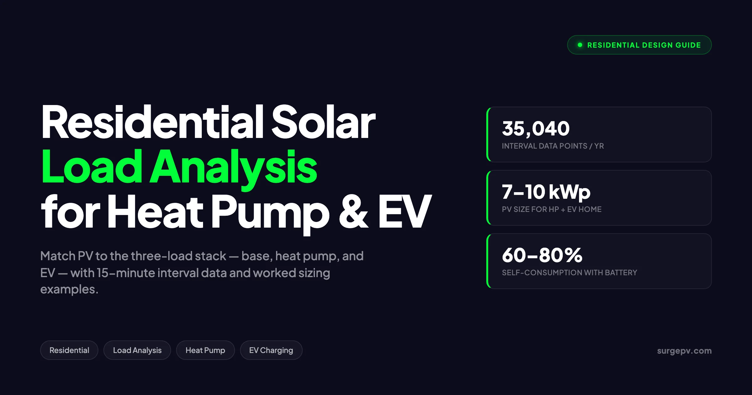
A typical UK or German household with both a heat pump and an EV uses 8,000 to 12,000 kWh of electricity per year — roughly three times what the same home consumed five years ago. Sizing a PV system to that profile using monthly bill totals is the single most common mistake in residential solar design today, and it leads to systems that either underperform in winter, export heavily in summer, or both. Residential solar load analysis is the discipline that fixes this, and the gap between a careful analysis and a back-of-envelope estimate now translates to thousands of euros over the life of a system. Also see: Us Residential Solar Market Trends 2026. For Germany-specific information, see Community Solar Projects Germany.
This is why every serious residential solar design tool — including SurgePV’s generation and financial tool — runs at 15-minute or hourly resolution. For a typical 3 to 4 person European household it averages 8 to 14 kWh per day with a clear evening peak between 6 PM and 10 PM. Also see: European Solar Tax Credits. For Europe-specific compliance details, see Europe solar compliance. For a direct comparison, see Arka 360 vs SurgePV.
This guide walks through the full analysis workflow that an experienced solar designer follows when a home has a heat pump, an EV, or both. You will see how to gather the right data, decompose the load into its three constituent layers, build an 8,760-hour profile, size PV and battery to match it, and forecast self-consumption with realistic numbers rather than vendor brochures. Worked examples cover three climates and three load configurations.
TL;DR — Residential Solar Load Analysis for HP and EV Homes
Use 15-minute interval data, not monthly bills. Decompose the load into base, heat pump, and EV layers — each has a distinct daily and seasonal shape. A 3 to 4 bedroom home with both loads typically needs 7 to 10 kWp of PV in Northern Europe (5 to 7 kWp in the US Sunbelt) plus 10 to 20 kWh of battery to reach 60 to 80 percent self-consumption. Scheduling matters more than nameplate capacity: EV charging shifted to midday lifts self-consumption by 15 to 40 percent with no extra hardware.
In this guide:
- What load analysis means and why monthly bills break down for HP and EV homes
- The three-load problem: base, heat pump, and EV layers
- Getting the right data: 15-minute intervals, Green Button, smart meters
- Heat pump load profiles by climate, system type, and control strategy
- EV charging profiles by charger level and owner behavior
- Building the combined 8,760-hour load stack
- Sizing PV to match the profile with three worked examples
- Battery sizing rules for combined HP and EV households
- Load shifting and smart control strategies
- ROI math and the most common sizing mistakes
What Is Residential Solar Load Analysis (and Why It Matters Now)
Load analysis is the process of decomposing and forecasting a home’s electricity consumption across time. For a basic resistive home — fridge, lights, appliances — a single annual kWh figure is usually enough to size a PV system. The shape of the load is predictable, daytime and evening peaks are modest, and any oversizing or undersizing shows up only at the margin.
Two changes have broken that approach. First, electrification has stacked two new high-power loads onto the same meter: hydronic or air-to-air heat pumps that pull 1 to 4 kW continuously through cold months, and Level 2 EV chargers that pull 7.2 to 11 kW for hours at a stretch. Second, time-of-use tariffs and self-consumption-based feed-in regimes mean the value of every exported kWh is now substantially less than the cost of every imported kWh — typically a 3 to 5x gap in Europe and a 2 to 3x gap in the US.
Together, these shifts mean that the time profile of consumption now matters as much as the annual total. A home that consumes 10,000 kWh per year with even hourly distribution wants a different system than a home that consumes 10,000 kWh per year with 60 percent of it falling between 5 PM and midnight. Both can be sized correctly. Neither can be sized correctly from the same monthly bill.
This is why every serious residential solar design tool — including SurgePV’s generation and financial tool — runs at 15-minute or hourly resolution. It is also why the upstream data collection step is non-negotiable: garbage in, garbage out, regardless of how sophisticated the simulation engine is.
Where Load Analysis Sits in the Design Process
Load analysis is the first technical step after the qualifying conversation with the homeowner. It precedes:
- PV array sizing and string layout
- Inverter selection and sizing
- Battery capacity and chemistry choice
- Shadow analysis and yield forecasting
- Self-consumption and ROI modeling
- Tariff selection and time-of-use optimization
Skipping load analysis or doing it superficially means every downstream decision is made on weaker ground. The cost of a thorough analysis is one to two hours of designer time. The cost of a wrong battery size is €4,000 to €10,000 of capital that never delivers the expected return.
The Three-Load Problem: Base Load, Heat Pump, EV
Modern residential load profiles for electrified homes have a layered structure. Treating them as a single curve obscures the design problem; decomposing them into three layers makes the design problem tractable.
Layer 1 — Base Load
The base load covers everything except heating and EV charging: refrigeration, lighting, cooking, electronics, ventilation, hot water (if not via heat pump), and small appliances. For a typical 3 to 4 person European household it averages 8 to 14 kWh per day with a clear evening peak between 6 PM and 10 PM. Annual base consumption usually falls in the 2,500 to 4,500 kWh range.
The base load is relatively predictable and changes slowly — it scales with household size, lifestyle, and appliance efficiency, but not with weather. In a load profile chart it appears as a steady ribbon that thickens at dinner time and overnight (refrigeration, base loads of always-on devices).
Layer 2 — Heat Pump
The heat pump layer is dominated by climate, system type, and house thermal envelope. A typical air-to-water heat pump for a 3 to 4 bedroom UK or German home consumes 3,000 to 6,000 kWh per year. Around 80 percent of that consumption falls between October 1 and March 31, with peaks in December, January, and February when ambient temperature drops and COP (coefficient of performance) falls below 3. See our guide on Heritage Building Solar Case Study for more. See our guide on MCS Certification for Solar Installers in the UK for more. For United Kingdom-specific compliance details, see United Kingdom comparisons/mcs-vs-non-mcs.
Within a winter day, heat pump load typically shows two peaks: an early-morning ramp (4 AM to 8 AM) as the system recovers setback temperatures, and an evening shoulder (5 PM to 9 PM) coinciding with occupancy and lower outdoor temperatures. Hot-water-only operation outside heating season produces a flatter, lower load — usually 200 to 400 kWh per month.
Air-to-air systems (Mitsubishi, Daikin ductless) and ground-source heat pumps follow similar seasonal patterns but with different daily shapes. Ground-source units run more steadily; ductless air-to-air units cycle harder and concentrate load when occupants are home.
Layer 3 — EV Charging
EV charging is the most behaviorally driven layer. A daily commute of 30 to 40 miles requires 8 to 12 kWh of charging, depending on the vehicle. A weekly 200 to 300 mile pattern adds 50 to 80 kWh per week. Long-distance drivers and two-EV households can push annual EV consumption to 4,000 to 6,000 kWh.
Charging shape depends on equipment and homeowner behavior:
- Level 1 (1.4 to 1.9 kW, 120V) — slow trickle, often overnight 8 to 12 hours; effectively a flat overnight ribbon
- Level 2 unscheduled (7.2 to 11 kW, 240V) — sharp evening peak from arrival until full, typically 5 PM to 9 PM
- Level 2 with timer (off-peak) — concentrated overnight pulse, often 1 AM to 5 AM under European cheap-rate tariffs
- Level 2 with solar diversion — daytime pulse, ramping with PV output, only usable when the home is unoccupied or the vehicle is parked during the day
The same annual kWh number under each of these four scenarios produces a completely different design problem. A home that reliably charges its EV between 11 AM and 3 PM during sunny months can effectively absorb 5 to 8 kW of midday PV that would otherwise be exported. A home that charges between 6 PM and 10 PM cannot absorb any of it without battery storage. See Adding Battery Storage Services for detailed guidance.
For a deeper look at this specific layer, see our guide to solar EV charging integration.
Why the Layered View Is Necessary
A combined load curve that just shows total kW over time is actually harder to design against than the three layers stacked. Stacking lets you ask the right questions in the right order:
- Is the base load matched well by daytime PV? (Almost always partially yes.)
- When does the heat pump run, and how much overlaps with PV production? (Usually little, especially in winter.)
- When does the EV charge, and is the charging window controllable? (Often yes, with the right charger.)
Each layer has different leverage. You can shift EV charging easily, heat pump operation moderately (with thermal storage or smart controls), and base load barely at all. Sizing decisions follow from this, not from a flat annual total.
Getting the Right Data: 15-Minute Intervals vs Monthly Bills
Load analysis quality is bounded by data quality. The available sources, in descending order of usefulness:
15-Minute Interval Data
The gold standard. A full year of 15-minute readings is 35,040 data points and contains every pattern that matters: evening peaks, weekday vs weekend differences, seasonal heating curves, EV charging spikes. This is the resolution that simulation tools like PV*SOL Premium 2026 and SurgePV’s generation and financial tool use natively.
How to get it:
- United States: Green Button Connect My Data through the utility customer portal. Most major utilities (PG&E, ConEd, SCE, ComEd, Duke) support direct download or API export of 15-minute interval data going back 12 to 24 months.
- United Kingdom: Smart meter data through the in-home display vendor app (Bright, Loop, Hugo) or directly from the supplier under the SMETS2 framework. n3rgy provides API access to half-hourly readings with consent.
- Germany: Smart meter rollout (intelligente Messsysteme) is incomplete; for homes without one, Bundesnetzagentur-certified gateway operators provide 15-minute readings on request.
- Other EU countries: National DSO portals (Enedis in France, e-distribución in Spain) provide free download of historical interval data with the meter PIN. Also see: Germany solar subsidies. Also see: France solar feed-in tariffs. Also see: Spain net metering.
Hourly Data
Acceptable but second-best. Hourly resolution captures most patterns but smooths out short-duration spikes — the very ones that drive battery sizing and inverter selection for EV-heavy homes. Hourly data is also what NREL’s PVWatts and most utility default exports provide. For more on this topic, see Inverter Selection Solar Design Guide.
Monthly Bills
Inadequate for HP and EV homes. Monthly totals can be back-fitted into a synthetic load profile using a regional reference shape, but the synthetic profile will systematically underestimate evening and winter peaks. For homes with no controllable loads, monthly data is workable; for any home with a heat pump, EV, or significant time-of-use exposure, it produces unreliable sizing.
Pre-Solar Baselines vs Post-Solar Behavior
A subtle trap: load patterns change after solar is installed. Homeowners with PV start running dishwashers, pool pumps, and EV charging during midday hours that they previously never used. The pre-installation load profile is the right starting point, but the post-installation simulation should account for a 10 to 20 percent shift of flexible loads to daytime hours if the homeowner is engaged.
For a deeper dive on interval data and synthetic profile construction, see our companion piece on solar system sizing with 15-minute interval load data.
Heat Pump Load Profiles — Hourly, Daily, Seasonal
The heat pump layer drives most of the seasonal mismatch in residential PV. Understanding its shape in detail is what separates a good design from a great one.
Annual Distribution by Month (Northern Europe Example)
For a 12 kW air-to-water heat pump serving a 150 m² UK home with average insulation:
| Month | Heating kWh | Hot Water kWh | Total kWh | Share of Annual |
|---|---|---|---|---|
| January | 720 | 120 | 840 | 19% |
| February | 620 | 110 | 730 | 16% |
| March | 480 | 110 | 590 | 13% |
| April | 280 | 100 | 380 | 8% |
| May | 110 | 90 | 200 | 4% |
| June | 30 | 80 | 110 | 2% |
| July | 0 | 80 | 80 | 2% |
| August | 0 | 80 | 80 | 2% |
| September | 60 | 90 | 150 | 3% |
| October | 280 | 100 | 380 | 8% |
| November | 480 | 110 | 590 | 13% |
| December | 250 | 120 | 370 | 8% |
| Total | 3,310 | 1,190 | 4,500 | 100% |
Note the asymmetric shape: 67 percent of consumption falls in the four months of November through February. PV production over those same four months in the UK is typically 12 to 15 percent of annual yield. The structural mismatch is roughly 5x.
Daily Profile by Season
Within a winter day, an air-to-water heat pump typically follows this pattern:
- 00:00 to 05:00 — overnight setback, low load (300 to 800 W)
- 05:00 to 09:00 — recovery ramp, peak draw (2 to 4 kW)
- 09:00 to 16:00 — maintenance load (500 W to 1.5 kW)
- 16:00 to 22:00 — evening occupancy peak (1.5 to 3 kW)
- 22:00 to 24:00 — pre-setback shoulder (1 to 2 kW)
In summer, the heat pump runs only for hot water, typically in two short pulses of 30 to 60 minutes each at 2 to 3 kW.
COP Drops in Cold Weather
A heat pump’s coefficient of performance falls as ambient temperature drops. A typical air-source unit operates at COP 3.5 to 4.0 at 7°C ambient and drops to COP 2.0 to 2.5 at -5°C. This means the same heat output requires 60 to 80 percent more electricity on cold days. The cold-weather electricity peak compounds the seasonal mismatch with PV — you need more kWh of input precisely when PV output is lowest.
Smart Controls and Thermal Storage
A heat pump with a smart controller and a buffer tank or thermal mass can shift 30 to 60 percent of its daily load into solar production hours. This is the single highest-leverage intervention available for HP-PV matching:
- Buffer tank (200 to 500 L) — lets the heat pump run hard during midday when PV is producing, storing heat for evening release
- Underfloor heating with thermal mass — slabs can be charged during midday to hold temperature into the evening
- Hot water priority during PV surplus — divert solar to the hot water cylinder before importing or exporting
For a system-level walk-through of HP-PV integration, see solar heat pump system design.
Pro Tip
If the home has a hydronic heat pump and underfloor heating, model the heat pump as 30 to 50 percent shiftable into PV hours rather than as a fixed load. The thermal mass of the slab effectively acts as a free battery for 4 to 8 hours of heating demand. This single modeling choice typically lifts forecast self-consumption by 8 to 15 percentage points without changing any hardware.
EV Charging Profiles — Schedules, Power Levels, Behavior
The EV layer is structurally simpler than the heat pump layer but more behaviorally variable. Three variables determine the profile: charger power, scheduling strategy, and weekly mileage.
Power and Energy Per Charge Session
| Charger | Power | 30-mile Top-up Time | 200-mile Recharge |
|---|---|---|---|
| Level 1 (120V, 12A) | 1.4 kW | 6.5 hours | 40+ hours |
| Level 1 (120V, 16A) | 1.9 kW | 5 hours | 30 hours |
| Level 2 (240V, 16A) | 3.8 kW | 2.5 hours | 15 hours |
| Level 2 (240V, 32A) | 7.7 kW | 75 minutes | 7.5 hours |
| Level 2 (240V, 48A) | 11.5 kW | 50 minutes | 5 hours |
| 3-phase (EU, 11 kW) | 11 kW | 50 minutes | 5 hours |
| 3-phase (EU, 22 kW) | 22 kW | 25 minutes | 2.5 hours |
Most home installs in Europe and the US settle on 7.2 kW (US single-phase) or 11 kW (EU three-phase). A typical commuter EV adds 8 to 15 kWh per day for 30 to 50 daily miles.
Charging Strategies and Their PV Implications
Plug-and-charge (no scheduling) — vehicle starts charging the moment it is plugged in, usually right after the homeowner gets home (5 to 7 PM). Worst case for solar self-consumption: zero overlap with PV production except in summer evenings. Annual self-consumption from EV layer alone: typically 0 to 10 percent without battery.
Off-peak timer (cheap rate window) — vehicle waits to charge during utility off-peak window (often 12:30 AM to 4:30 AM in the UK on Octopus Go or similar). Zero solar self-consumption from EV; instead optimizes against grid tariff structure. This is the most common UK setup today.
Solar-aware charging (PV diversion) — smart charger (Zappi, Wallbox Quasar, Tesla Wall Connector with Powerwall) modulates current to match PV surplus. EV charges when there is excess solar, pauses or trickles when there is not. Self-consumption from EV layer can reach 60 to 80 percent if the vehicle is parked at home during daylight.
Time-of-use plus solar arbitrage — charges from solar when available, from grid only at off-peak rates. Most sophisticated and best economic outcome but requires the right hardware and an engaged homeowner.
For homeowners who can shift charging to daytime, see our vehicle-to-grid (V2G) and solar design coverage on the next-generation use case.
EV Load Profile Examples
Commuter (single EV, plug-and-charge):
- Daily: 12 kWh consumed between 6 PM and 8 PM
- Weekly: ~85 kWh
- Annual: 4,300 kWh
Two-EV household (one daytime, one overnight):
- Daytime EV (work-from-home spouse): 6 kWh between 11 AM and 1 PM
- Overnight EV: 10 kWh between 1 AM and 4 AM
- Combined annual: 5,800 kWh
Solar-diversion single EV:
- Charges 4 to 8 kWh per day from PV surplus, May to September
- Charges 8 to 12 kWh per night from off-peak grid, October to April
- Combined annual: 3,900 kWh, of which 1,200 kWh from solar surplus
The same annual mileage produces wildly different design implications under each profile.
Combined Load Stack: Building the 8,760-Hour Profile
Once you have the three layers characterized, the combined load stack is the sum of the three at each 15-minute or hourly timestep across a full year. This 8,760-hour (or 35,040-quarter-hour) profile is the input to the simulation.
Construction Steps
- Start with measured base load from interval data, ideally from a period before HP and EV were installed. If only post-installation data is available, subtract estimated HP and EV usage by analyzing typical-day shapes.
- Layer the heat pump model using a degree-day or hour-by-hour thermal model, calibrated against billing data if available. Free models from degreedays.net work well; commercial tools (PV*SOL, Polysun) include built-in HP libraries.
- Layer the EV model based on stated charging schedule and weekly mileage. Account for seasonal range loss (15 to 30 percent winter range reduction in cold climates).
- Validate the combined profile against actual annual consumption ± 10 percent. If it deviates further, revisit the assumptions in the layer with the largest uncertainty.
Why Modeling Each Layer Separately Pays Off
A single combined curve cannot answer the most important design questions: “What if the homeowner shifts EV charging to daytime?” “What if a buffer tank lets the heat pump run during PV peak?” “What if a battery is sized to cover the evening base load only?” Each of these scenarios changes one layer at a time. A modular load stack lets you re-simulate quickly; a flat curve forces you to start over.
This is also why load profile analysis is treated as a discipline distinct from load total estimation in commercial PV — and the same logic now applies to electrified residential systems.
Run the load stack in SurgePV in under 10 minutes
Import 15-minute interval data, layer heat pump and EV profiles, and simulate PV + battery sizing across the full 8,760 hours.
Book a DemoNo commitment required · 20 minutes · Live project walkthrough
Sizing PV to Match the Load — Three Worked Examples
The right PV size depends on climate, load shape, controllable load fraction, and the homeowner’s economic objective (maximize self-consumption, minimize bill, maximize ROI). Three worked examples cover the typical decision space.
Example 1 — UK Family Home, Heat Pump and Single EV
- Location: Manchester, UK
- Roof: South-facing, 30° pitch, 35 m² usable
- Annual consumption: 9,800 kWh (4,500 HP + 4,300 EV + 1,000 base)
- EV charging: plug-and-charge, evenings
- Heat pump: standard hydronic, no buffer tank
- Tariff: Octopus Go (4-hour cheap window 00:30-04:30)
Sizing decision:
| PV Size | Annual Yield | Self-Consumption | Bill Saving | Payback |
|---|---|---|---|---|
| 4 kWp | 3,600 kWh | 65% (2,340 kWh) | £820/yr | 9.5 yr |
| 6 kWp | 5,400 kWh | 50% (2,700 kWh) | £960/yr | 10.5 yr |
| 8 kWp | 7,200 kWh | 40% (2,880 kWh) | £1,050/yr | 12 yr |
| 8 kWp + 10 kWh battery | 7,200 kWh | 75% (5,400 kWh) | £1,820/yr | 11 yr |
The 8 kWp + 10 kWh combination delivers the best total bill saving and a competitive payback. Without the battery, scaling above 6 kWp produces diminishing returns because midday production is exported.
Example 2 — German Single-Family Home, HP + 2 EVs
- Location: Munich, Germany
- Roof: East-west split, 25° pitch, 60 m² usable
- Annual consumption: 12,500 kWh (5,500 HP + 6,000 2x EV + 1,000 base)
- EV charging: one daytime (work-from-home), one overnight
- Heat pump: ground source with 400 L buffer tank
- Tariff: standard residential, EEG feed-in for surplus
Sizing decision:
| PV Size | Annual Yield | Self-Consumption | Bill Saving | Payback |
|---|---|---|---|---|
| 8 kWp | 7,600 kWh | 60% (4,560 kWh) | €1,420/yr | 8 yr |
| 10 kWp | 9,500 kWh | 52% (4,940 kWh) | €1,560/yr | 8.5 yr |
| 12 kWp | 11,400 kWh | 45% (5,130 kWh) | €1,640/yr | 9 yr |
| 10 kWp + 15 kWh battery | 9,500 kWh | 78% (7,410 kWh) | €2,580/yr | 9 yr |
The combination of the daytime EV and the buffer-tank-equipped heat pump means even the no-battery 10 kWp option achieves over 50 percent self-consumption. The battery still pays off, but the marginal benefit is smaller than in the UK example because the load already overlaps better with PV production.
Example 3 — US Sunbelt Home, HP + EV
- Location: Phoenix, Arizona
- Roof: South-facing, 18° pitch, 60 m² usable
- Annual consumption: 14,200 kWh (5,800 HP cooling + 4,400 EV + 4,000 base AC)
- EV charging: Level 2 unscheduled, evening
- Cooling load dominates summer; heat pump for both heating and cooling
- Tariff: TOU (4-9 PM peak, all other hours off-peak)
Sizing decision:
| PV Size | Annual Yield | Self-Consumption | Bill Saving | Payback |
|---|---|---|---|---|
| 7 kWp | 12,200 kWh | 55% (6,710 kWh) | $1,650/yr | 8 yr |
| 9 kWp | 15,700 kWh | 45% (7,065 kWh) | $1,780/yr | 8.5 yr |
| 9 kWp + 13.5 kWh battery | 15,700 kWh | 80% (12,560 kWh) | $2,820/yr | 9 yr |
In TOU markets the peak-shifting value of a battery is substantial — the battery does not just lift self-consumption, it also displaces the most expensive grid hours. This dynamic does not appear in the European examples because EU tariffs are typically flat or only modestly time-differentiated.
Sizing Heuristic by Region
For a quick first-pass sizing, use these regional rules of thumb for an electrified home (HP + 1 EV):
| Region | PV (kWp) per 1,000 kWh load | Battery (kWh) per kWp PV |
|---|---|---|
| UK / Ireland | 0.75 | 1.5 |
| Germany / Benelux | 0.85 | 1.5 |
| France / N. Spain | 0.65 | 1.0 |
| S. Spain / Italy / Greece | 0.50 | 1.0 |
| US Northeast | 0.85 | 1.5 |
| US Sunbelt | 0.55 | 1.5 |
| US Mountain West | 0.65 | 1.0 |
These ratios assume south-facing or east-west pitched roofs with limited shading. For shaded or split roofs, increase PV by 15 to 25 percent. For tracker-mounted ground systems, decrease by 10 to 15 percent.
Battery Sizing for Combined HP + EV Households
Battery sizing is where the most expensive sizing mistakes happen. The simple rule “match daily consumption” produces oversized, expensive batteries that never reach payback. The right approach uses the load stack and asks how much capacity actually displaces grid imports at the price the battery cycle costs.
The Cost-of-Cycled-Energy Constraint
A residential lithium battery in 2026 has a levelized cost of cycled energy (LCOCE) of €0.08 to €0.12 per kWh in Europe and $0.10 to $0.14 per kWh in the US, accounting for capital cost, cycle life, and round-trip efficiency. A battery cycle only adds value if the spread between import price and export price exceeds the LCOCE. In practice this means:
- UK with Octopus Go (~£0.30 import / £0.15 export): spread is £0.15, so battery cycles pay
- Germany with EEG feed-in (~€0.32 import / €0.08 export): spread is €0.24, batteries pay strongly
- Spain with PVPC self-consumption (~€0.25 import / €0.08 export): spread is €0.17, batteries pay
- US with net metering 1:1: spread is zero, batteries do not pay
- US with NEM 3.0 (CA, ~$0.40 import / $0.07 export): spread is $0.33, batteries pay strongly
Sizing Rule for HP + EV Homes
Start with this heuristic:
Battery capacity (kWh) = 1.0 to 1.5 × evening base load + 0.5 × heat pump evening load + 0 × EV (handle EV separately with smart charger)
For a typical UK home with a heat pump and an EV:
- Evening base load (5 PM to midnight): ~4 kWh
- HP evening load (winter): ~6 kWh
- Battery target: 6 to 9 kWh
Cap at 1.5 to 2 kWh per kWp PV — beyond this ratio, the battery sits empty too often to pay off.
For homes with a buffer-tank-equipped heat pump and a daytime-charged EV, the battery target drops further because both layers overlap with PV. For homes with no controllable loads, the battery target rises but rarely above 15 to 20 kWh in residential settings.
Why “Cover One Day of Backup” Is the Wrong Frame
Homeowners often ask for a battery that covers one day of consumption. For a 9,800 kWh/year UK home, that suggests 27 kWh of battery — which would be twice as expensive as needed and would never reach full discharge in summer. Backup capability is a distinct sizing exercise (covered in our commercial battery storage sizing piece, with logic that scales down to residential), and conflating it with self-consumption sizing inflates costs without adding value.
Battery and Heat Pump Co-Location
A subtle but important point: in winter, the battery should generally not be used to feed the heat pump from PV-charged cycles. The math rarely works because winter PV generation is too low to keep the battery topped up, and using grid-charged battery cycles to feed a heat pump just adds round-trip losses to grid power. The battery’s job in winter is to serve evening base load and the household electronics layer; the heat pump should run primarily on direct grid or direct PV (when available).
For deeper coverage of the battery sizing question across system types, see battery solar system design for the UK.
Load Shifting and Smart Controls — Lift Self-Consumption Without More Panels
The cheapest kWh of self-consumption is the one that comes from rescheduling a controllable load, not from adding hardware. Three control strategies deliver most of the available gain.
EV Charging Diversion
A solar-aware EV charger (Zappi, Wallbox Quasar, Tesla Wall Connector with Solar) modulates charge current to track PV surplus. When the home is exporting more than 1.4 kW, the charger ramps up; when the home is importing, it pauses or drops to a minimum.
Impact: 15 to 40 percentage point lift in EV-layer self-consumption if the vehicle is parked at home during daylight. Hardware cost is €600 to €1,200 for a smart charger versus €400 to €700 for a basic Level 2 unit. Payback is typically 18 to 36 months on the incremental cost.
Heat Pump PV Synchronization
Modern heat pumps with SG Ready (Smart Grid Ready) inputs accept signals from the inverter or energy management system to ramp up production when surplus PV is available. Combined with a buffer tank or thermal mass, this shifts 30 to 60 percent of daily heat pump load into solar hours.
Impact: 8 to 15 percentage point lift in HP-layer self-consumption. Implementation requires an SG Ready-capable heat pump (most premium units sold since 2020), a buffer tank or thermal mass, and an energy management system that can issue the signal. Software-only retrofits exist for some units (Daikin Onecta, Mitsubishi Melcloud, Vaillant sensoNET).
Hot Water Diversion
Resistive immersion heaters in a hot water cylinder act as a natural sink for surplus PV. A diverter (myenergi Eddi, Solar iBoost) sends excess generation to the immersion element instead of exporting it. For homes without a heat pump for hot water, this is the simplest and cheapest control intervention.
Impact: 5 to 12 percentage point lift in total self-consumption. Hardware cost €350 to €600. Payback typically 2 to 4 years.
Combined Effect
A home with all three controls and a properly sized battery can reach 80 to 90 percent self-consumption — within a few percentage points of off-grid operation, at a fraction of the off-grid system cost. The same system without controls typically tops out at 55 to 65 percent regardless of battery size.
This is the single largest gap between “what the brochure says” and “what the system actually delivers.” Designers who model controls realistically deliver systems that match their forecast; designers who model loads as fixed deliver systems that disappoint.
For more on the rules and tariff structures behind self-consumption value across Europe, see solar self-consumption rules in Europe.
ROI Math: What HP + EV Households Actually Save
The financial case for residential solar in HP + EV homes is structurally stronger than in conventional homes because the imported electricity being displaced is larger. But the case depends entirely on getting the sizing right.
Bill Reduction Components
For the UK example above (8 kWp + 10 kWh battery, 75 percent self-consumption):
| Item | Annual kWh | Unit Value | Annual Value |
|---|---|---|---|
| Direct PV consumption | 5,400 | £0.30 (avoided import) | £1,620 |
| Battery time-shifted PV | 0 (already counted) | — | — |
| Exported surplus | 1,800 | £0.15 (SEG) | £270 |
| Reduced peak demand charges | — | n/a | £0 |
| Total annual benefit | £1,890 |
System cost (8 kWp PV + 10 kWh battery, installed): £14,500. Payback: 7.7 years on bill savings alone, before any maintenance or replacement costs. IRR over 25 years (assuming 4 percent annual electricity inflation): 11 to 13 percent.
The same home with no battery and a 4 kWp system: bill saving £820/yr, system cost £6,800, payback 8.3 years. Comparable absolute payback but much lower lifetime value.
Sensitivity to Tariff Structure
ROI is heavily sensitive to import-export tariff spread. The same system in three jurisdictions:
| Market | Import Price | Export Price | Annual Saving | Payback |
|---|---|---|---|---|
| UK (SEG, Octopus) | £0.30 | £0.15 | £1,890 | 7.7 yr |
| Germany (EEG) | €0.32 | €0.08 | €2,180 | 7.5 yr |
| Spain (PVPC) | €0.25 | €0.07 | €1,720 | 9.5 yr |
| California (NEM 3.0) | $0.40 | $0.07 | $2,920 | 6.5 yr |
| Texas (no net metering) | $0.13 | $0.04 | $980 | 16 yr |
The pattern: jurisdictions with high retail prices and meaningful self-consumption incentives produce strong returns. Markets with low electricity prices or unfavorable export terms produce weak returns regardless of how good the load analysis is.
For a deeper financial analysis with country-by-country detail, see solar panel ROI in Italy and our European solar incentives guide.
Common Sizing Mistakes to Avoid
The same handful of mistakes account for most residential PV underperformance in HP + EV homes.
Mistake 1 — Sizing on Annual kWh
Symptom: a 10 kWp system on a UK home that exports 6,000 kWh/year and still pays £700/year for winter electricity. Cause: annual totals hid the seasonal mismatch.
Fix: model the load and PV at hourly resolution before committing to any size.
Mistake 2 — Treating EV Charging as Fixed Schedule
Symptom: design assumes EV charges from solar at midday; homeowner actually plugs in at 6 PM and charges through the evening. Self-consumption reaches 35 percent instead of forecast 65 percent.
Fix: design around the actual charging behavior or provide the smart charger as part of the install.
Mistake 3 — Oversizing the Battery
Symptom: 20 kWh battery on a UK home, only fully charges 30 days per year, never fully discharges in winter. Battery pays off in 14 years on a 12-year warranty.
Fix: size battery against evening load, not daily load. Cap at 1.5 to 2 kWh per kWp PV.
Mistake 4 — Ignoring Heat Pump COP Curve
Symptom: forecast HP consumption based on rated COP (3.5); actual winter COP averages 2.4; HP consumes 45 percent more than modeled.
Fix: use temperature-binned COP data from the manufacturer’s datasheet, not nameplate COP.
Mistake 5 — Designing for Today’s Load, Not Tomorrow’s
Symptom: home gets a second EV 18 months after install; system was right-sized for one EV and is now undersized.
Fix: ask the homeowner about likely additions in the next 5 years (second EV, hot tub, pool, ducted AC, basement office). Add 15 to 25 percent headroom if any are realistic. The marginal cost of bigger PV at install is much lower than the cost of an upgrade later.
Conclusion
For homes with a heat pump and an EV, residential solar load analysis is no longer optional — it is the controlling step in design quality, and the load profile feeds directly into the financial model in solar proposal software. Three concrete actions for any installer or designer working in this space:
- Always pull 15-minute interval data before sizing. Monthly bills have failed for HP + EV homes; treat them as a backup, not a primary source.
- Model the load in three layers (base, HP, EV) and treat the controllability of each separately. The decision to add a smart EV charger or HP buffer tank often beats the decision to add a kWp of panels.
- Use the cost-of-cycled-energy framework to size batteries, capped at 1.5 to 2 kWh per kWp of PV. The “cover one day” rule belongs to backup sizing, not self-consumption sizing.
Run these three steps consistently and the gap between forecast and actual performance closes from the typical 15 to 25 percent range to under 5 percent — which is what turns a satisfied customer into a referring one.
Frequently Asked Questions
What is residential solar load analysis?
Residential solar load analysis is the process of mapping a home’s electricity consumption across hours, days, and seasons before sizing a PV system. It typically uses 15-minute interval meter data (35,040 readings per year) to expose patterns that monthly bills hide, including evening peaks, winter heating loads, and EV charging windows. The analysis is the foundation for every downstream decision: PV size, battery capacity, inverter selection, and self-consumption forecasts.
How many solar panels do I need for a heat pump and an EV?
A typical 3 to 4 bedroom home with one heat pump and one EV consumes 8,000 to 12,000 kWh per year, which usually requires a 7 to 10 kWp PV system in Northern Europe and 5 to 7 kWp in Southern Europe or the US Sunbelt. The exact number depends on roof orientation, climate, EV mileage, and whether the heat pump runs hydronic or air-to-air. Without a battery, a 7 kWp system on a UK home with both loads achieves roughly 30 to 40 percent self-consumption.
Why does heat pump load matter for solar sizing?
Heat pumps consume around 80 percent of their annual electricity between October and March, when solar output is at its lowest. That seasonal mismatch is the single biggest reason a home with a heat pump cannot rely on annual kWh totals for sizing. A system that looks balanced on paper may still draw heavily from the grid in January and export aggressively in July.
Should I size PV to cover EV charging fully?
Only if the EV charges during daylight hours or you have battery storage. A typical EV adds 8 to 15 kWh per day, but most owners charge overnight on Level 2 chargers that draw 7.2 kW. Without scheduling or a battery, the PV system will export midday surplus and the EV will pull from the grid at night. Smart EV chargers that pause until solar is available change the math substantially.
What battery size do I need with a heat pump and EV?
For a 3 to 4 person Central European household with both loads, 15 to 20 kWh of usable battery capacity covers most evenings outside winter and lifts self-consumption from roughly 30 percent to 65 to 80 percent. In the UK and Northern Europe, larger batteries do not meaningfully help in midwinter because solar production is so low. The cost-effective ceiling is usually 1.5 to 2 kWh of battery per kWp of PV.
What interval data do I need to do a proper load analysis?
The gold standard is 15-minute interval data covering at least one full year, ideally exported through Green Button or a similar utility portal. Hourly data is acceptable if the home does not have time-of-use rates or significant short-duration loads. Monthly bills are not enough to size systems with heat pumps or EVs because they hide the evening and seasonal peaks that drive battery and inverter decisions. Solar design software automates design and compliance.