Quick Answer
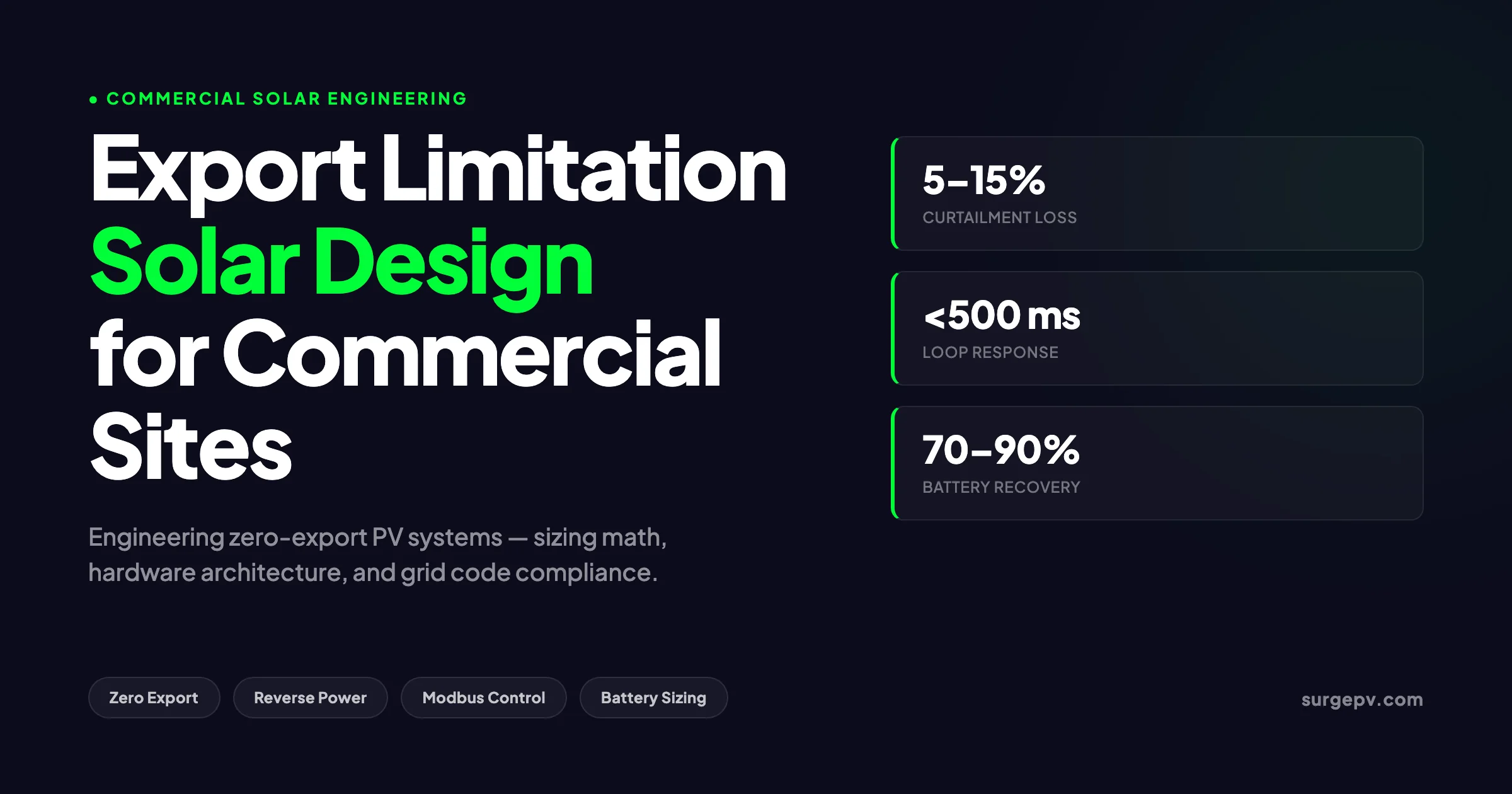
Commercial export-limited solar systems use smart inverters, zero-export devices, and battery storage to prevent grid feed-in where net metering is unavailable or capped. Typical design: oversized DC array (1.2–1.4x AC rating) with energy storage to absorb excess generation. Cost premium: 5–15% versus standard grid-tied systems.
Half of all distributed PV interconnection studies in 2025 ended with an export limit attached to the approval. That number comes from the DOE i2X interconnection roadmap update (DOE, 2025), and it reframes the design problem. For a growing share of commercial sites, the question is no longer how much PV the roof can hold — it is how much PV the meter will let onto the grid. Export limitation has shifted from a niche workaround to a core engineering deliverable on three- and four-out-of-five C&I projects.
Commercial export-limited solar systems use smart inverters, zero-export devices, and battery storage to prevent grid feed-in where net metering is unavailable or capped. Typical design: oversized DC array (1.2–1.4x AC rating) with energy storage to absorb excess generation. Cost premium: 5–15% versus standard grid-tied systems. For more on this topic, see Adding Battery Storage Services.
Commercial export-limited solar systems use smart inverters, zero-export devices, and battery storage to prevent grid feed-in where net metering is unavailable or capped. Typical design: oversized DC array (1.2–1.4x AC rating) with energy storage to absorb excess generation. Cost premium: 5–15% versus standard grid-tied systems.
This guide covers the full engineering workflow for export-limited and zero-export commercial PV. It walks through control architecture, hardware selection, sizing math under an export cap, response time tuning, multi-inverter clustering, and commissioning tests. The numbers and protocols here apply to systems from 50 kW to 5 MW on commercial and industrial sites under utility export caps from full feed-in down to absolute zero.
TL;DR
Export limitation is a closed-loop control system that caps grid feed-in at a configured setpoint, including absolute zero. The design workload is real — load profile analysis, controller selection, response time tuning, and battery sizing — but well-executed zero-export systems lose only 5 to 15 percent of theoretical generation on most commercial loads. The economic case beats waiting 12 to 24 months for an unrestricted interconnection on a constrained feeder.
In this guide:
- The three export limitation modes — static, dynamic, and absolute zero — and when each applies
- Why utilities impose export caps on commercial connections, with grid code references for the US, EU, UK, Australia, and India
- Hardware architecture — meters, current transformers, gateways, and inverter requirements
- The 8-step zero-export design workflow, from load profile to commissioning
- Sizing math under an export cap, including a worked 500 kW commercial example
- Battery storage sizing for curtailment recovery, with a payback comparison
- Communication protocols and response time tuning for grid code compliance
- Multi-inverter and multi-injection-point control strategies
- Commissioning and acceptance test procedures
- Eight common export limitation design mistakes and how to avoid them Also see: Best Solar Design Software India.
What Export Limitation Means and the Three Modes
Export limitation is a continuous control loop that measures power flow at the point of common coupling and adjusts inverter output to keep grid feed-in below a configured setpoint. The setpoint is not always zero. It is a number — sometimes 100 percent of inverter nameplate, sometimes 30 percent, sometimes a strict zero with a few hundred watts of tolerance.
Three modes cover almost every commercial deployment.
Static Export Limit
The simplest mode. The inverter is configured with a fixed kW cap that it will never exceed, regardless of on-site load. A 500 kW PV system with a 200 kW static export limit will output up to 200 kW to the grid plus whatever the on-site load consumes. The cap is a constant, not a dynamic value.
Static limits suit installations with predictable surplus profiles or sites where the utility wants a guaranteed maximum injection regardless of behind-the-meter activity. They are easy to commission — set a value, lock it. They are also the least efficient because they do not use available headroom on the on-site load.
Dynamic Export Limit
The setpoint is fixed but the actual injection adjusts in real time based on on-site consumption. If the site is drawing 150 kW and the inverter would otherwise produce 400 kW, the inverter caps at 150 kW plus the export setpoint. As the load varies through the day, the inverter follows it.
Dynamic limits use the full available headroom under the cap. They require a CT or revenue meter at the service entrance and a fast control loop. Most modern string and central inverters support this mode out of the box — SolarEdge, SMA, Huawei, Sungrow, and Fronius all ship it as a firmware option. Use the generation and financial tool to model how much of your generation actually clears the export cap under a dynamic limit.
Zero Export
The absolute case. The setpoint is zero or a small dead-band like 1 kW. The inverter never exports surplus. Any on-site under-consumption causes immediate curtailment. Grid codes in some markets require absolute zero — Italy’s Resolution 5/24 ARG/elt, the Indian SECI guidelines for net metering deniers, and a number of UK DNO export-zero connection offers. Also see: solar panel ROI in Italy. For India-specific information, see 5kW Solar Panel Price in India. For India-specific compliance details, see India andhra-pradesh.
Zero export is the strictest design constraint because the optimization target changes. Without storage, useful generation is capped by the daytime load floor — the lowest hourly demand during the solar window. Sites with a flat 200 kW daytime load and a 500 kW PV array will lose 60 percent of theoretical generation. Sites with a clean match between load and irradiance lose under 10 percent.
Pro Tip
Always read the connection offer carefully. The phrase “no export” can mean different things across utilities — some allow a small spillover for measurement noise, some require literal zero with a 200 W trip threshold. The control loop tuning differs significantly between a 1 kW dead-band and a 200 W dead-band.
Why Utilities Impose Export Caps on Commercial Connections
Export limits exist because the local low-voltage and medium-voltage networks were not built for reverse power flow at the scale of modern PV penetration. Five constraints drive the cap.
Transformer Backfeed
Distribution transformers are sized for one-way power flow from the substation to the load. When PV exports exceed local demand, current reverses through the transformer. Most LV transformers handle this without damage at low penetration, but high export volumes cause overheating, accelerated insulation aging, and tap-changer wear. The DSO Frontier Network technical paper from CIGRE 2024 documented a 30 percent reduction in transformer service life on feeders with backfeed exceeding 50 percent of nameplate (CIGRE, 2024). For Australia-specific compliance details, see Australia comparisons/lgc-vs-stc.
Voltage Rise
Pushing power up an LV cable raises voltage at the injection point. EN 50160 caps steady-state voltage at +10 percent of nominal, and individual DSOs often set tighter operational limits at +6 to +8 percent. A 500 kW PV system on a long rural LV feeder can lift voltage above the limit at the inverter terminals, tripping the system or violating the grid code. Export limitation keeps voltage within band by capping injection.
Protection Coordination
Distribution protection schemes assume current flows from substation to fault. Reverse current from PV can mask faults, delay protection trip times, or cause unintended operation of directional relays. Above a certain penetration, the utility either upgrades the protection scheme or limits export. Limiting is cheaper.
Capacity Allocation
Many utilities allocate feeder capacity on a first-come-first-served basis. When a feeder is at capacity, new connections come with export caps to avoid further loading. This is the dominant driver in dense urban C&I markets — London, Berlin, Mumbai, Sydney inner-west. For the latest details on Germany, see Community Solar Projects Germany. Read Community Solar Business Model for a complete walkthrough.
Tariff Structure
In markets without net metering or with strict net billing, export earns nothing or earns a price below avoided cost. The owner has no economic incentive to export and the utility has no incentive to accept it. A zero export configuration is the cleanest commercial outcome for both parties.
The five drivers stack. A single project can hit transformer constraints and voltage rise and protection coordination simultaneously, and the utility issues a zero export connection offer rather than running three separate engineering studies.
Grid Code References by Market
Export limitation rules are written into national grid codes and DSO connection conditions. The references below cover the major commercial PV markets.
| Market | Standard | Export Limit Provisions |
|---|---|---|
| United States | IEEE 1547-2018, UL 1741-SB | Inverter must support external power limit command. Specific limits set by interconnection agreement and Rule 21 (CA), 2030.5 (national). |
| Germany | VDE-AR-N 4105, VDE-AR-N 4110 | Static curtailment to 70 percent of nameplate for systems below 25 kW. Dynamic curtailment via FRT/FRC for larger systems. |
| United Kingdom | G99 Annex A.5, ENA EREC G100 | Export limitation scheme required for systems above DNO threshold. G100 is the standard reference for export limit design. |
| Australia | AS/NZS 4777.2:2020 | Dynamic export controls under DER Register. Setpoint changes within 5 seconds. Loss of setpoint trips inverter within 10 seconds. |
| Italy | CEI 0-16, CEI 0-21 | RTU-based external curtailment for medium-voltage connections. Zero export available under SCAMBIO SUL POSTO end-of-life. |
| Spain | RD 244/2019 | Self-consumption with simplified surplus or compensation. Zero export common for systems above 100 kW. |
| India | SECI guidelines, state DISCOM regulations | Zero export mandatory in many states under net billing. Reverse power relay required at PCC. |
| Brazil | ANEEL Resolution 1000/2021 | Export caps tied to compensation tier. Mini-generation up to 5 MW with simplified review. |
The detailed national rules are covered in the grid export limitation rules by country post. For the underlying engineering definition, see the grid export limitation glossary entry.
Hardware Architecture for Export-Limited Commercial PV
A commercial export limitation system has four hardware blocks. Get any of them wrong and the control loop either runs too slow, runs out of headroom, or misreads the meter and trips the system.
Block 1 — Meter or Current Transformers at the Point of Common Coupling
The system needs to know real-time grid power flow with directional awareness. Two options.
Bi-directional revenue-grade meter. A three-phase Class 0.5 or Class 1 meter installed at the service entrance, downstream of the utility meter. The meter outputs power flow values via Modbus RTU or TCP. Examples — Carlo Gavazzi EM340, Janitza UMG 96RM, Eastron SDM630.
Current transformers plus a power analyzer. Three split-core or solid-core CTs around the incoming phases, wired to a power analyzer or directly to the inverter’s CT input. This is cheaper and faster, with bandwidth of about 50 ms versus 500 ms for Modbus meters.
For commercial sites above 100 kW, use revenue-grade CTs with 0.5S accuracy. Below 100 kW, retrofit-grade CTs are usually acceptable.
Block 2 — Zero Export Controller or Gateway
The brain of the loop. Reads meter or CT values, compares to setpoint, and issues power limit commands to the inverters. Three options.
Inverter-native control. Modern string inverters from SolarEdge, SMA, Huawei, Sungrow, and Fronius accept CT inputs directly and run the export control loop in firmware. No external gateway needed for single-inverter sites or homogeneous clusters.
Vendor gateway. SolarEdge SetApp, SMA Sunny Home Manager / Cluster Controller, Huawei SmartLogger, Sungrow Logger1000, Fronius Smart Meter — each vendor ships a gateway that handles cluster-level export control and meter aggregation. Use these when the site has multiple inverters from the same vendor.
Vendor-agnostic gateway. Elum ePowerControl, Janitza UMG controllers, Trina Tracker NCU, custom PLCs running IEC 61131-3 logic. Required when the site has mixed inverter brands or when the controller must integrate with a SCADA system. These cost 1.5 to 3x more than vendor gateways but handle any inverter that exposes a Modbus power limit register.
Block 3 — Communication Backbone
Three protocols dominate.
Modbus RTU over RS-485. Daisy-chain wiring, up to 32 nodes per segment without a repeater, baud rates from 9600 to 115200. Most commercial inverters expose their power limit registers over Modbus RTU. Latency is 50 to 300 ms per command depending on baud rate and node count.
Modbus TCP over Ethernet. Star topology via switch, theoretically unlimited nodes, latency under 50 ms. Use for sites with existing structured cabling or for greater than 32-inverter clusters. Requires either dedicated VLAN or industrial firewall to keep PV control traffic separate from corporate IT.
SunSpec Modbus profile. A standardized register map maintained by the SunSpec Alliance. Most modern inverters speak SunSpec for the common power limit and status registers, which lets a vendor-agnostic gateway control mixed brands without custom register tables. Verify SunSpec compliance via the alliance’s test results database before committing to a multi-vendor cluster design.
Block 4 — Inverter with External Power Limit Support
Not every inverter accepts external power limit commands. The minimum requirements:
- Power limit register. A Modbus holding register that, when written, immediately reduces the inverter’s AC output to the commanded value.
- Setpoint timeout. The inverter must trip or fall back to a safe state if the setpoint is not refreshed within a configured time window. AS/NZS 4777.2 requires 10 seconds. Most grid codes accept 30 seconds.
- Ramp rate control. Optional but recommended. The inverter ramps to the new setpoint over a configured period rather than stepping instantaneously, which reduces flicker.
Older inverters without external power limit support cannot be retrofitted into a zero export system without an upstream curtailment device — usually a contactor on the AC side that disconnects the inverter when grid power approaches zero. This is a poor solution because it loses all PV generation during the disconnect, not just the surplus.
For new commercial designs, use solar design software that maintains an inverter compatibility database with export limit support flags. SurgePV’s database tracks the power limit register, ramp rate range, and setpoint timeout for every commercial inverter from SMA, SolarEdge, Huawei, Sungrow, Fronius, GoodWe, and others.
The 8-Step Zero Export Design Workflow
A clean zero export design moves through eight steps. Skipping any of them shows up later as either commissioning failures or curtailment surprises in the first month of operation.
Step 1 — Load Profile Analysis
Pull at least 12 months of 15-minute or 30-minute interval data from the site’s revenue meter. The data drives every downstream sizing decision. Three statistics matter most.
- Daytime load floor. The 5th percentile of demand during the solar window (06:00 to 18:00 local time). This is the upper bound of useful PV without storage under a zero export limit.
- Daytime average load. The mean demand during the solar window. This is what the system will hit on most clear-sky days.
- Weekend versus weekday delta. Many commercial sites drop to a 10 to 30 percent baseline on weekends. A 500 kW Monday load can become a 50 kW Sunday load.
Plot the data as a heat map — hour of day on x-axis, day of year on y-axis. The visualization shows seasonal load patterns and weekend dips at a glance.
Step 2 — Irradiance and Generation Profile
Pull TMY3 or PVGIS hourly irradiance data for the site coordinates. Convert to expected hourly generation using a draft system size — module rating, tilt, azimuth, system losses. Match the generation profile against the load profile from Step 1.
The overlap area is useful generation. The generation above the load is curtailment. The load above the generation is grid import.
Step 3 — Set the Curtailment Tolerance
Decide how much curtailment loss the project can absorb. Three reference points.
- Under 5 percent. Excellent match. Either the load is highly correlated with irradiance, the system is sized below the load floor, or there is significant battery storage.
- 5 to 15 percent. Typical for a well-designed commercial system without storage on a daytime-active site.
- Above 15 percent. Either the system is oversized, the load is weekend-idle, or storage is mandatory to make the economics work.
Run the generation and financial tool with the load profile and irradiance data to find the system size that hits the target curtailment.
Step 4 — Select the Control Architecture
Choose between vendor-native control, vendor gateway, or vendor-agnostic gateway. The decision rests on three questions.
- How many inverters? Single-inverter sites use native control. Multi-inverter sites need a gateway.
- Single brand or mixed? Mixed brands force a vendor-agnostic gateway.
- SCADA integration? Sites with plant SCADA need a controller that supports IEC 61850 GOOSE or a Modbus-to-DNP3 bridge.
Step 5 — Specify the Meter and CTs
Match meter accuracy to the cap. A 200 W zero export dead-band needs Class 0.5 meters with 0.2S CTs. A 1 kW dead-band tolerates Class 1 meters with 0.5 CTs.
Locate the meter on the line-side of any non-export load that should not count toward consumption. Common mistake — placing the CT on the wrong side of a backup generator transfer switch, which double-counts generator output during testing.
Step 6 — Tune the Control Loop
Three parameters need sign-off before commissioning.
- Setpoint. The export cap in kW. Usually zero for a zero export system. Some grid codes allow a small positive value to absorb measurement noise — confirm with the DSO.
- Dead-band. The window around the setpoint where the controller does not act. A 1 kW dead-band around a 0 kW setpoint means the controller acts on +1 kW export but not on +0.5 kW.
- Response time. The time from detected violation to throttled output. Set to the fastest the protocol supports, typically 200 to 500 ms for Modbus and under 100 ms for hardwired CT.
Step 7 — Battery Storage Sizing (If Applicable)
If curtailment exceeds the tolerance from Step 3, add storage. Size the battery to capture the curtailed kWh on a typical clear-sky day, not the worst case. Sizing for the worst case overspends by 30 to 50 percent for a marginal improvement in annual yield.
A clean rule — battery kWh capacity equals 0.6 to 0.8 times the daily curtailed kWh. Round-trip efficiency of 85 to 92 percent puts useful recovery at 70 to 90 percent of curtailment.
Step 8 — Commissioning and Acceptance Test
The final design step is the commissioning plan. Document the test sequence, expected response times, pass thresholds, and the rollback procedure if the test fails. The full commissioning protocol is covered later in this guide.
Sizing Math Under an Export Cap — A Worked 500 kW Example
A worked example makes the math concrete. The site is a metal fabrication plant in Manchester, UK, with the following parameters. For the latest details on UK, see Battery Solar System Design UK.
| Parameter | Value |
|---|---|
| Annual electricity consumption | 1,950,000 kWh |
| Average daytime load (06:00–18:00) | 280 kW |
| Daytime load floor (5th percentile) | 145 kW |
| Weekend load | 60 kW average |
| Roof available for PV | 3,800 m² |
| Annual irradiance (Manchester) | 950 kWh/m²/yr |
| DNO export offer | Zero export under G100 |
Without Storage
The load floor sets the upper bound for non-curtailed PV size. At 145 kW load floor, a 200 kW DC system on a clear summer day will see 145 kW absorbed by the load and 55 kW curtailed. The annual curtailment depends on the distribution of load and irradiance hours.
A simulation with hourly TMY data and the actual 30-minute load profile gives:
- 200 kW DC system — 178,000 kWh useful, 12,000 kWh curtailed (6.3 percent loss)
- 300 kW DC system — 248,000 kWh useful, 36,000 kWh curtailed (12.7 percent loss)
- 400 kW DC system — 305,000 kWh useful, 75,000 kWh curtailed (19.7 percent loss)
- 500 kW DC system — 348,000 kWh useful, 127,000 kWh curtailed (26.7 percent loss)
The right size without storage is between 250 and 300 kW DC, where the loss stays under the 15 percent tolerance and the project still delivers ~250 MWh/year.
With Storage
Adding a 300 kWh battery shifts the math significantly. The curtailed kWh on summer days runs 700 to 1,200 kWh. The battery captures 300 kWh of that and discharges into the evening load, displacing grid import.
- 500 kW DC system + 300 kWh battery — 410,000 kWh useful, 65,000 kWh curtailed (13.7 percent loss after storage)
- 500 kW DC system + 500 kWh battery — 440,000 kWh useful, 35,000 kWh curtailed (7.4 percent loss after storage)
The battery moves the system from a 26.7 percent loss to a 7.4 percent loss, recovering 92,000 kWh per year. At a UK commercial electricity price of £0.27/kWh, that is £24,840 per year. A 500 kWh LFP battery system at £180/kWh installed cost is £90,000, putting payback at 3.6 years.
Run the Numbers on Your Export-Limited Site
SurgePV’s design platform models load profiles, curtailment, and battery sizing in one workflow. Export the financial case for an export-limited project in under 30 minutes.
Book a DemoNo commitment required · 20 minutes · Live project walkthrough
Battery Sizing for Curtailment Recovery
Battery sizing for export-limited systems differs from sizing for time-of-use arbitrage or backup. The goal is to capture surplus PV during the curtailment window and discharge during the import window. Three sizing methods.
Method 1 — Daily Curtailment Average
Take the average daily curtailment in kWh from the simulation. Multiply by 0.7. The result is a battery size that captures most curtailment without paying for low-utilization capacity.
For the 500 kW Manchester example, average summer daily curtailment is 600 kWh. A 420 kWh battery captures most of it. Round to a standard size — 400 kWh.
Method 2 — 90th Percentile
Size to the 90th percentile of daily curtailment, not the maximum. The maximum corresponds to a few sunny weekend days where load is lowest and irradiance is highest. Sizing to the 90th percentile keeps utilization high and avoids paying for capacity that runs at low cycle count.
Method 3 — Self-Consumption Target
Set a target self-consumption ratio — say 75 percent — and back out the battery size. This works when the design constraint is a contractual self-consumption percentage rather than a curtailment percentage.
For all three methods, the battery should also be sized to handle the inrush during morning ramp-up. A 500 kW PV system on a clear morning ramps from 0 to 500 kW in roughly 2 hours. The battery needs C/2 charge capability or the system curtails through the ramp.
The detailed battery sizing methodology is covered in the commercial battery storage sizing guide.
Communication Protocols and Response Time Tuning
The control loop has four legs — meter to controller, controller to inverter, inverter ramp time, and feedback to meter. Total loop latency is the sum.
Modbus RTU (RS-485)
Typical commercial deployment. 19200 or 38400 baud. 8N1 framing. Multidrop wiring with up to 32 nodes per segment.
- Meter to controller — 100 to 200 ms per polling cycle
- Controller to inverter — 50 to 200 ms per command
- Inverter ramp — 100 to 500 ms depending on ramp rate setting
- Total loop — 250 ms to 1 second
Tune by raising baud rate to 115200 if cable length allows, reducing polling cycle to 100 ms, and setting inverter ramp rate to maximum (or removing it for tightest control).
Modbus TCP (Ethernet)
Higher performance, higher cost. Typical loop times under 200 ms.
- Meter to controller — 20 to 50 ms
- Controller to inverter — 20 to 50 ms
- Inverter ramp — same as RTU
- Total loop — 150 to 400 ms
Use TCP for sites with more than 32 inverters, sites already wired with Ethernet, or sites where the SCADA system is TCP-native.
Hardwired Analog (4-20 mA)
Fastest. The meter outputs 4-20 mA proportional to grid power, the inverter accepts 4-20 mA on its analog input, and the loop runs at the meter’s sample rate.
- Loop time — under 50 ms
- Wiring — twisted shielded pair, point to point
- Drawback — only one inverter per loop without analog multiplexing
Use for single-inverter sites with strict response time requirements (under 200 ms).
Setpoint Timeout
Every grid code requires the inverter to fall back to a safe state if the setpoint command is lost. Configure the timeout to match the regulator’s requirement.
| Region | Required Timeout | Typical Setting |
|---|---|---|
| AS/NZS 4777.2 (Australia) | 10 seconds | 8 seconds |
| G100 (UK) | 30 seconds | 20 seconds |
| VDE-AR-N 4105 (Germany) | 60 seconds | 30 seconds |
| IEEE 1547-2018 (US) | Per interconnection agreement | 30 seconds default |
The fallback state can be either trip-to-zero or curtail-to-zero — confirm the requirement in the connection conditions.
Multi-Inverter and Multi-Injection-Point Control
Single-inverter sites are easy. Multi-inverter and multi-injection-point sites need careful attention to how the limit command is divided.
Single-Point Injection, Multi-Inverter
The site has one PCC and multiple inverters all feeding into the same bus. The controller reads grid power at the PCC and divides the limit command across inverters.
Two strategies for division.
Equal share. The controller sends the same limit command to every inverter. Simple, but fails when one inverter has a fault — the others do not pick up the slack. Use only on identical, redundant clusters.
Proportional share. The controller monitors each inverter’s actual output and divides the limit proportional to current production. Better behavior under partial fault — if one inverter trips, the others ramp up to fill the gap up to the cap. Default for most modern gateways.
Multi-Point Injection
The site has multiple PCCs — typically a campus with separate buildings, each with its own utility connection. Each PCC has its own meter and its own export limit. The controller has to enforce the limit at each point independently.
Two architectures.
Federated. Each PCC has its own controller and meter, and the local controller manages the inverters on that bus. The PCCs are independent.
Centralized. One controller polls all PCC meters and issues commands to all inverters across all buses. More flexible — surplus from a low-load building can be redirected to a high-load building if the grid topology allows. Requires a higher-spec controller and a wider communication backbone.
Most multi-PCC commercial sites use federated control because the grid topology rarely allows surplus redirection — the buses are physically separate from the utility’s perspective.
Generator and Storage in the Same Site
Sites with backup generators or battery storage need extra logic. The controller has to distinguish between PV export, battery export, and generator export. Wire the meter to read net power flow at the PCC and use the controller’s source-of-export logic to allocate the cap correctly.
Common mistake — placing the meter inside the load loop and missing the battery’s discharge contribution. The fix is to wire the meter at the actual utility boundary and let the controller compute net flow.
Commissioning and Acceptance Test Procedure
The acceptance test proves the export limit holds under realistic conditions. Run the test before grid energization sign-off.
Pre-Energization Checklist
- All CTs and meters wired with correct phase rotation. Verify with a phase rotation meter.
- All inverter Modbus addresses unique and registered with the controller.
- Setpoint, dead-band, ramp rate, and timeout configured per design.
- Communication backbone tested with a manual ping from the controller to every inverter.
- Inverter firmware version meets minimum for export limit support — check the manufacturer’s release notes.
Test 1 — Steady-State Limit
Bring the system online during a clear-sky daytime hour. Confirm grid power at the PCC stays at or below the setpoint for 15 minutes. Record the dead-band utilization — the actual oscillation around the setpoint.
Pass — grid power within dead-band for 99 percent of samples.
Test 2 — Load Step Response
Drop a major on-site load (turn off a chiller or process line). Measure the time from load drop to inverter throttle. Compare to the spec.
Pass — throttle complete within 1 second for Modbus systems, 200 ms for hardwired.
Test 3 — Setpoint Timeout
Disconnect the controller from the inverters. Confirm all inverters trip or curtail to zero within the configured timeout window.
Pass — all inverters reach safe state within timeout +1 second.
Test 4 — Inverter Fault Recovery
Trip one inverter manually. Confirm the remaining inverters do not exceed the cap during the trip and the system rebalances within 5 seconds.
Pass — no export violation during fault, system rebalanced within 5 seconds.
Test 5 — 24-Hour Trend
Leave the system running for 24 hours with full data logging. Pull the trend log. Look for spurious export events, oscillation around the setpoint, and missed throttle commands.
Pass — no export above the setpoint plus the dead-band, no setpoint command failures.
Document every test result with timestamps and meter values. The DSO will often request the trend log as part of the connection sign-off package.
Eight Common Export Limitation Design Mistakes
The same eight mistakes show up across most failed export limit commissioning runs. Avoiding them is the cheapest improvement available to a commercial design team.
Mistake 1 — Sizing for Average Load Instead of Load Floor
Designers anchor on average daytime demand. The system gets sized to 280 kW for a site with 280 kW average load. The 5th percentile drops to 145 kW, and the system curtails 30 percent of generation on light-load days.
Fix — anchor sizing on the 5th percentile load floor. Use the average only as an upper bound for systems with battery storage.
Mistake 2 — Wrong Side of the Generator Transfer Switch
The CT goes on the building side of the generator ATS instead of the utility side. During testing, the controller reads generator output as load and lets PV inject. The fix is obvious but the mistake repeats on every site with a backup generator.
Fix — always place the CT or meter at the utility-facing side of any source transfer device.
Mistake 3 — Mixing Inverter Brands Without SunSpec Compliance
The site has two SMA Tripowers and two Huawei SUN2000s. The cluster controller is a vendor-agnostic gateway. Commissioning fails because one of the inverter firmware revisions does not implement the SunSpec immediate power limit register correctly.
Fix — verify SunSpec compliance for the exact firmware version on every inverter before specifying a vendor-agnostic gateway. When in doubt, default to single-vendor clusters.
Mistake 4 — Setting the Dead-Band Too Tight
The DSO requires zero export with a 200 W tolerance. The designer sets the dead-band to 0 W. The control loop oscillates ±300 W around zero, occasionally crossing into export. The DSO trips the connection during a routine audit.
Fix — set the dead-band to half the DSO tolerance, with the setpoint biased into the import direction by another quarter of the tolerance. For a 200 W tolerance, set dead-band to 100 W and setpoint to -50 W (50 W into import).
Mistake 5 — Ignoring Ramp Rate
The inverter ramp rate is set to default (typically 10 percent per minute). On a load drop, the inverter takes 10 minutes to throttle from 500 kW to zero. Half of that ramp pushes power into the grid above the cap.
Fix — set the inverter ramp rate to the highest supported value, or disable ramping entirely for export limit applications. Confirm flicker compliance separately.
Mistake 6 — No Battery Pre-Charge Logic
The battery sits idle through the morning ramp because the controller logic only charges from “surplus” — which is a curtailment trigger. By the time curtailment starts, the battery is empty and the morning ramp curtails on the inverter rather than the battery.
Fix — implement pre-charge logic that uses the irradiance forecast to start charging before curtailment triggers. Most modern energy management systems support this natively.
Mistake 7 — Communication Failure Mode Untested
The Modbus cable gets disconnected during a maintenance event. The controller stops responding. The inverters wait for the timeout and then trip. Production drops to zero for the rest of the day, even though the underlying issue was a 30-second cable disconnect.
Fix — test the communication failure mode as part of commissioning. Set the timeout to the longest value the DSO accepts. Implement a reconnection retry that resumes operation if communication restores within a configurable window.
Mistake 8 — No Trend Logging
The system runs for six months without a single audit. Then the DSO calls about a complaint from a neighboring building. There is no trend log to defend against the complaint. The connection gets pulled.
Fix — log every meter reading, setpoint command, and inverter response at 1-minute resolution to a non-volatile store. Retain at least 12 months of data. This is the cheapest insurance available against DSO disputes.
ROI and Economic Impact of Export Limitation
Export limitation changes the economic calculus in three ways.
Curtailment Cost
The first-order cost is the lost generation. A 5 to 15 percent curtailment loss translates directly to a 5 to 15 percent reduction in annual revenue from PV. On a 500 kW commercial system at £0.20/kWh self-consumption value, 10 percent curtailment is roughly £10,000 per year.
Avoided Interconnection Upgrade
The first-order benefit is avoiding the network upgrade that would otherwise be required to allow full export. Network upgrades on constrained UK feeders run £200,000 to £2,000,000. The export limit lets the system connect immediately without the upgrade.
Connection Timeline
The second-order benefit is timeline. An unrestricted commercial connection on a constrained feeder can take 12 to 24 months. An export-limited connection often takes 3 to 6 months. The 9 to 18 month timeline difference is worth £30,000 to £100,000 in production for a 500 kW system, plus the avoided cost of capital tied up during the wait.
Battery Storage Payback
When curtailment exceeds 15 percent, battery storage pays back fast. Using the Manchester worked example — a 500 kWh LFP battery at £90,000 captures £25,000 per year of curtailed energy, paying back in 3.6 years. The same battery on a site without an export limit would pay back in 7 to 10 years through TOU arbitrage alone.
The export limit is, paradoxically, the best economic case for adding storage to a commercial site. It compresses the payback timeline by half or better.
Pro Tip
If the DSO offers a choice between a 50 percent dynamic export limit and a 0 percent zero export limit with a 50 percent network upgrade contribution, run the math. Many sites end up better off with the zero export limit and a battery — the battery captures most of the curtailed energy and the project avoids the upgrade contribution entirely.
Software Workflow for Export-Limited Designs
Modern solar design platforms ship export limitation modeling as a first-class feature. The workflow integrates load profile import, irradiance simulation, curtailment calculation, battery sizing, and inverter cluster control configuration into a single project.
The solar design software and solar proposal software workflow for an export-limited project runs in five stages.
- Project setup — Import the site location, roof geometry, and load profile. Match the load profile to the local utility’s interval data format (e.g., 30-minute kWh in CSV).
- System sizing — Run the design engine with the export cap as a constraint. The software returns the optimal DC nameplate, string configuration, and inverter selection that maximizes useful generation under the cap.
- Curtailment modeling — Simulate hourly generation against the load profile. Output the curtailed kWh and the percentage loss for each candidate system size.
- Storage sizing — Add battery options. Re-run the simulation with charge and discharge logic to find the storage size that hits the curtailment tolerance at the lowest CapEx per recovered kWh.
- Proposal and documentation — Generate the customer proposal with the curtailment chart, payback math, and the controller architecture diagram. Export the inverter and gateway BOM directly into the procurement system.
The workflow that used to take a week in spreadsheets and standalone PVsyst runs now compresses to half a day. Use Clara AI to suggest curtailment-tolerant sizings and storage options based on the load profile. For software options, see 7 Best PVsyst Alternatives in.
Conclusion
- Anchor sizing on the load floor, not the average. The 5th percentile of daytime demand is the upper bound for non-curtailed PV without storage. Most sizing mistakes start with the wrong reference number.
- Verify SunSpec or vendor compatibility before specifying a multi-vendor cluster. Mixed-brand zero export systems work when every inverter implements the standard registers correctly, and fail when any one of them does not.
- Run the 5-test acceptance protocol before grid sign-off. Steady-state, load step, setpoint timeout, inverter fault, and 24-hour trend. The DSO will eventually ask for the test results — having them in hand from day one shortens every audit and protects the connection.
Frequently Asked Questions
What is export limitation in a commercial solar system?
Export limitation is a control strategy that caps the amount of power a PV system can push back to the utility grid. The inverter monitors a current transformer or revenue meter at the point of common coupling, and ramps down DC production whenever export approaches the configured setpoint. Limits range from full export, to a fixed kW cap, to absolute zero export.
How does a zero export solar system work?
A zero export system uses a bi-directional energy meter at the service entrance to measure net power flow. When the meter detects current flowing toward the grid, a controller signals the inverter to throttle output via Modbus or hardwired analog control. Response time is typically 200 milliseconds to 2 seconds depending on the protocol, which is fast enough to keep export within grid code tolerances.
What hardware do you need for a zero export commercial PV system?
The minimum hardware stack is a three-phase bi-directional energy meter or current transformers at the point of common coupling, a zero export controller or gateway, and at least one inverter that supports external power limit commands. For multi-inverter sites you also need a daisy-chain communication backbone, typically Modbus RTU over RS-485 or Modbus TCP over Ethernet.
How much energy do you lose to a zero export limit?
Curtailment loss depends on the load profile and system sizing. A well-matched zero export system on a commercial site with daytime load typically loses 5 to 15 percent of theoretical generation. Mismatched systems on weekend-idle sites can lose 40 percent or more. Adding battery storage recovers 70 to 90 percent of curtailed energy in most commercial designs.
What is the response time required for zero export inverters?
Most grid codes require export to be reduced within 2 seconds of detecting a violation. Modern Modbus-controlled inverters respond in 200 to 500 milliseconds. Hardwired analog control loops respond in under 100 milliseconds. AS/NZS 4777.2 in Australia requires export setpoint changes to take effect within 5 seconds, and the inverter must trip if the setpoint is lost for more than 10 seconds.
Can you do zero export with multiple inverters?
Yes. The zero export controller reads total grid power at the point of common coupling and divides the limit command across all inverters in the cluster. Each inverter then enforces its share of the limit locally. SMA, SolarEdge, Huawei, Sungrow, and Fronius all support cluster-level export control through proprietary gateways or open Modbus profiles.
Is export limitation the same as anti-islanding?
No. Anti-islanding disconnects the inverter when the grid is lost. Export limitation throttles inverter output while the grid is energized. Both functions are required by IEEE 1547 and most national grid codes, and both run continuously in parallel — anti-islanding is a fail-safe trip, while export limitation is a continuous power control loop.
Does zero export design change the optimal system size?
Yes. Without export, the optimization target shifts from maximum annual kWh to maximum useful kWh. The system should be sized to the daytime load floor for the lowest curtailment, or oversized with battery storage to capture surplus. A commercial site with 200 kW average daytime load might cap PV at 220 to 250 kW DC without storage, or scale to 400 kW DC with a 500 kWh battery.