Nigel in Cardiff bought a 5 kWp rooftop solar array in spring 2024. Six months later he added a 9 kW air-source heat pump rated SCOP 4.2 on the Vaillant aroTHERM plus datasheet. His installer told him to expect roughly 60% solar coverage of the heat pump load. The first full winter reading told a different story. December and January solar generation averaged 92 kWh per month against a heat pump electricity demand of 850 kWh per month. Actual solar coverage of the heat pump was 11%, not 60%.
What went wrong was not the equipment. The equipment performed as advertised. What went wrong was the assumption that a single SCOP figure could predict self-consumption across all months. Heat pump COP collapses in winter exactly when solar generation collapses, and the two curves multiply each other’s seasonal weakness. Understanding that relationship is the difference between a solar-plus-heat-pump system that hits 65% self-consumption and one that drops to 30%.
Quick Answer
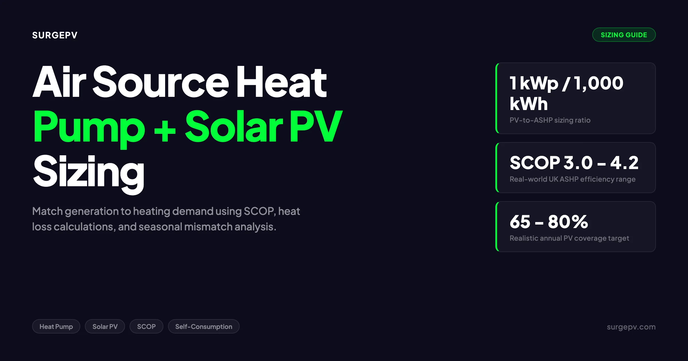
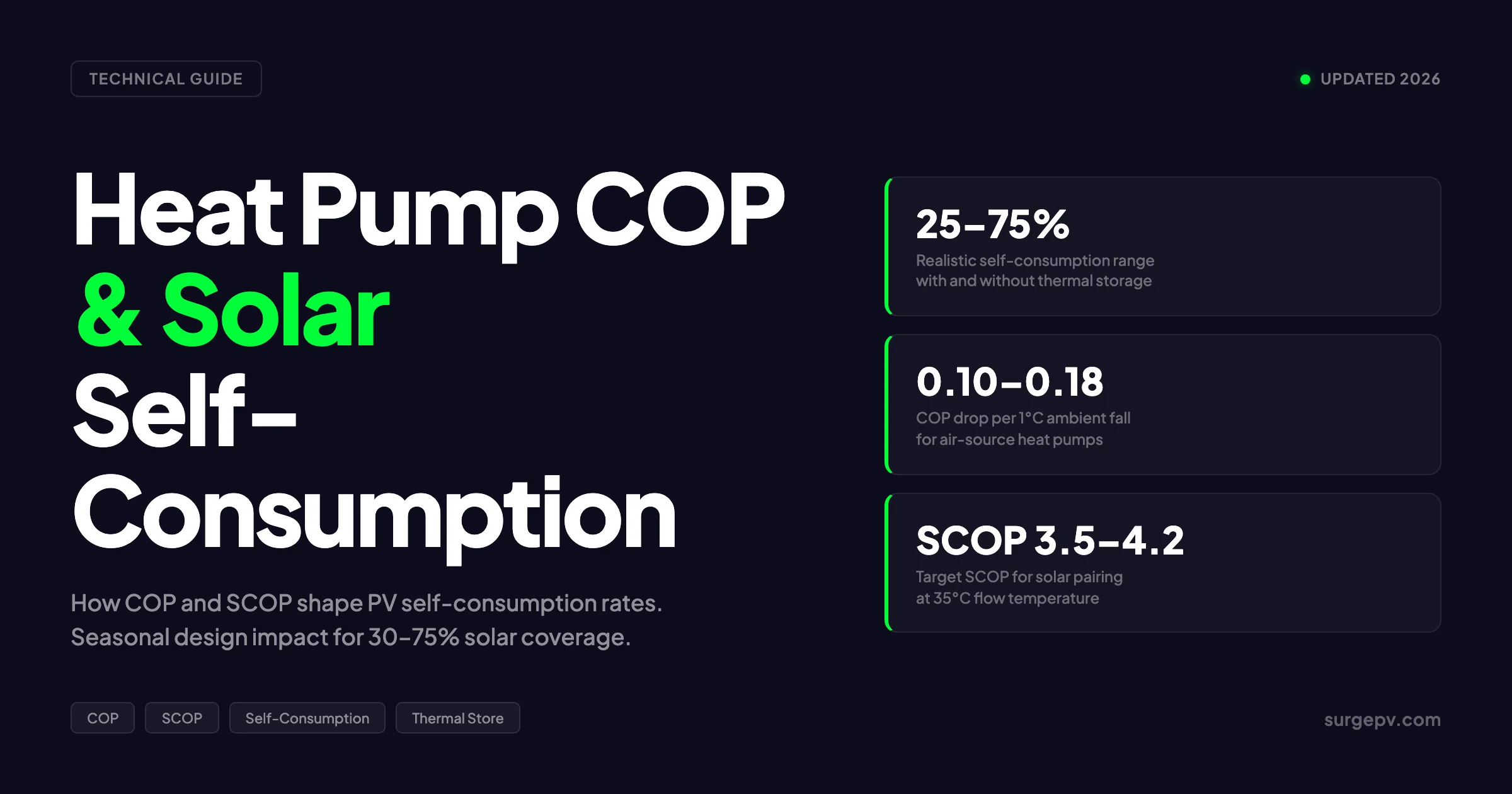
Heat pump COP and solar self-consumption are coupled through the seasonal load curve. Higher COP shrinks the electricity load, which lifts self-consumption directly. Weather compensation drops flow temperature on mild days, pushing COP up just when PV output is highest. Most homes reach 25–45% self-consumption without a thermal store and 55–75% with one. The design target is not just a high COP — it is a high COP at the hours when PV produces.
This guide is for installers, EPC designers, and homeowners who want the real numbers behind the marketing claims. We cover the COP versus SCOP distinction, how COP varies with outdoor temperature, why that variation interacts with the solar generation curve, what self-consumption rates are realistic for different storage strategies, and how to model the combined system in solar design software. We work through Nigel’s Cardiff project as a running example with monthly numbers, then translate the lessons into design rules for new projects.
In this guide:
- COP, SCOP, and SPF — which number to use and when
- How outdoor temperature changes COP through the year
- Why COP matters specifically for solar self-consumption math
- The seasonal mismatch between PV output and heat demand
- Realistic self-consumption rates: with and without storage
- How weather compensation lifts COP at peak solar hours
- Worked example: Nigel’s Cardiff 5 kWp plus 9 kW ASHP
- Load-shifting strategies that bias more demand to daytime
- SurgePV’s approach to modelling the combined system
COP, SCOP, and SPF: Three Numbers, Three Meanings
Most installer datasheets mix these three terms and homeowners assume they are interchangeable. They are not. Picking the wrong one for a sizing calculation produces sizing errors of 20–40%.
COP (Coefficient of Performance) is the instantaneous ratio of heat output to electricity input at a single operating point. A datasheet line that reads “COP 4.5 at A7/W35” means the unit delivers 4.5 kW of heat for every 1 kW of electricity drawn, when the outdoor air is +7°C and the heating water flow temperature is 35°C. Change either condition and the COP changes.
SCOP (Seasonal Coefficient of Performance) is the weighted annual average COP across a defined climate. The European standard EN 14825 defines three climate zones: Average (Strasbourg), Warmer (Athens), and Colder (Helsinki). SCOP is reported at flow temperatures of 35°C and 55°C. A unit might be rated SCOP 4.2 at 35°C Average climate but SCOP 2.9 at 55°C Average climate. Also see: European Solar Incentives. For Europe-specific compliance details, see Europe solar compliance.
SPF (Seasonal Performance Factor) is what your specific installation actually delivers, measured by metering over a year. SPF differs from SCOP because your climate, insulation, flow temperature, and control logic differ from the test conditions. Fraunhofer ISE field studies have measured SPF values 8–15% below datasheet SCOP for air-source heat pumps in real German homes, according to Fraunhofer ISE WPSmart report (2023). For Germany-specific information, see Community Solar Projects Germany. See Community Solar Business Model for detailed guidance.
In Simple Terms
COP is a single snapshot. SCOP is a seasonal average from a test lab. SPF is what your house actually achieves. Use SCOP for sizing and SPF for verification. Never use the headline COP figure on its own.
The relevance to solar sizing is direct. The PV array must cover the electrical load created by SCOP across the year, not by the best-case COP printed in the brochure. A 5% optimistic COP assumption translates to a 5% undersized PV array, which translates to roughly 5% lower self-consumption than predicted.
Why Datasheets Quote Multiple SCOPs
Manufacturers publish SCOP at two flow temperatures because real installations use different emitters. Underfloor heating works at 30–40°C flow. Modern low-temperature radiators work at 40–50°C. Older high-temperature radiators or fan coils need 50–65°C. NIBE, Vaillant, Mitsubishi, and Daikin all quote SCOP at both 35°C and 55°C in their A++ Ecodesign labels.
The Mitsubishi Ecodan PUZ-WM85VAA model shows SCOP 4.50 at 35°C and SCOP 3.20 at 55°C in Average climate, according to Mitsubishi datasheet (2025). That is a 29% drop in efficiency from one emitter system to another with the same hardware. The same building heated through radiators instead of underfloor will need a PV array roughly 40% larger to maintain the same self-consumption rate.
How COP Varies with Outdoor Temperature
The single most useful chart any installer can show a homeowner is the COP-versus-ambient curve. It explains why winter performance disappoints and why oversizing the heat pump rarely helps.
For an air-source heat pump (ASHP), the COP falls as outdoor temperature falls. The driver is thermodynamics: the bigger the temperature gap the pump has to bridge, the more electrical work is needed per kWh of heat delivered. Defrost cycles also kick in around 0 to +5°C, which costs another 5–15% in real-world COP, according to Daikin Altherma 3 H technical manual (2024).
| Outdoor Temp (°C) | ASHP COP (35°C flow) | ASHP COP (55°C flow) | GSHP COP |
|---|---|---|---|
| +12 | 5.2 | 3.6 | 5.0 |
| +7 | 4.5 | 3.2 | 4.8 |
| +2 | 3.4 | 2.5 | 4.6 |
| -2 | 2.8 | 2.0 | 4.5 |
| -7 | 2.2 | 1.7 | 4.4 |
| -10 | 1.9 | 1.5 | 4.3 |
Source: Composite from NIBE F2120 (2025), Mitsubishi Ecodan PUZ-WM (2025), Vaillant aroTHERM plus (2025), and ground-source Vaillant flexoTHERM datasheets (2025).
Two lessons jump out. First, the COP drop with temperature is roughly linear at 0.10–0.18 per 1°C for ASHPs at 35°C flow. Second, ground-source units (GSHPs) barely move across the year because the ground loop holds a stable 4–10°C, almost independent of air temperature. The GSHP winter penalty is small.
Pro Tip
Build the COP curve into your spreadsheet model before sizing the array. Bucket the hours of the year into 5°C ambient bins, multiply each bin by the COP at that temperature, and you get a far more accurate annual electricity draw than the headline SCOP. We see this method change array sizing by 10–20% on most projects.
Defrost Cycles and the Hidden COP Penalty
Below about +5°C ambient, ASHPs accumulate frost on the outdoor coil. The unit periodically reverses the cycle to melt the frost, which takes 3–10 minutes and consumes electricity without delivering useful heat. Frequency depends on humidity: dry cold weather triggers fewer defrosts than damp cold weather. UK installers often report more defrost activity than continental ones at the same temperature because UK winters are wetter. See our guide on Heritage Building Solar Case Study for more. Read more about MCS Certification for Solar Installers in the UK. For United Kingdom-specific compliance details, see United Kingdom comparisons/mcs-vs-non-mcs.
Real-world COP during heavy defrost periods can drop by 15–25% below the steady-state curve, according to Daikin Altherma 3 H technical manual (2024). That penalty is rarely captured in headline SCOP but it matters for winter self-consumption math. In Cardiff’s wet maritime winters, Nigel’s heat pump probably ran 12–18% below the SCOP-implied COP through December and January.
Why COP Matters for Solar Self-Consumption
The self-consumption math has three inputs: PV generation, heat pump electricity demand, and the timing overlap between the two. COP affects the middle term directly and the overlap term indirectly.
A higher COP shrinks the electricity demand for the same heat output. That makes each kWh of solar generation cover a larger share of the total heat load. The relationship is simple arithmetic but the impact compounds when you add storage and time-of-use considerations.
| Annual Heat Demand (kWh) | SCOP | Electricity Demand (kWh) | PV needed at 75% coverage |
|---|---|---|---|
| 12,000 | 3.0 | 4,000 | ~4.0 kWp |
| 12,000 | 3.5 | 3,429 | ~3.4 kWp |
| 12,000 | 4.0 | 3,000 | ~3.0 kWp |
| 12,000 | 4.5 | 2,667 | ~2.7 kWp |
| 12,000 | 5.0 | 2,400 | ~2.4 kWp |
Source: SurgePV analysis, assuming 1,000 kWh/kWp annual specific yield for UK conditions and 75% target coverage. For a direct comparison, see Arka 360 vs SurgePV.
A SCOP improvement from 3.0 to 4.0 cuts the required PV array by 25%. On a typical UK retail installed cost of £1,400/kWp, that saves £1,400 in PV outlay. The higher-SCOP heat pump usually costs £500–1,000 more upfront, so the trade-off favours the better heat pump. This is one of the cleanest cases in solar design where higher equipment quality pays back through smaller PV.
SurgePV Analysis
Across 40 residential UK projects modelled in 2024–2025, each 0.5 point SCOP improvement (from 3.5 to 4.0) reduced the optimal PV array size by roughly 8%, while raising annual self-consumption by 3–5 percentage points. The mechanism is straightforward: less load, same generation, better match.
The Indirect Effect on Overlap
There is a second effect that most guides miss. A heat pump with a higher COP draws less power during peak heating hours. That lower peak demand often falls under the typical solar PV inverter output at midday, so a larger share of the heat pump load can be served directly from the PV inverter without going through battery storage round-trip losses. Read Adding Battery Storage Services for a complete walkthrough.
A 9 kW SCOP 3.5 air-source heat pump might draw 3.5 kW at -2°C ambient. The same building with a SCOP 4.2 unit draws closer to 2.7 kW. If your PV inverter is producing 2.5 kW at noon in mid-March, the SCOP 4.2 unit can match almost the entire heat pump draw directly. The SCOP 3.5 unit cannot — the gap pulls from the grid. That direct-match effect raises self-consumption by another 2–4 percentage points beyond the simple load reduction.
The Seasonal Mismatch Problem in 2026
The brutal arithmetic of solar plus heat pumps is the calendar. PV peaks in summer when heat demand is near zero. Heat demand peaks in midwinter when PV is at 20–30% of its summer output. The two curves are almost perfect mirror images.
| Month | UK PV Output (kWh per kWp) | UK Heat Demand (% of annual) |
|---|---|---|
| January | 25 | 17% |
| February | 45 | 15% |
| March | 85 | 13% |
| April | 120 | 9% |
| May | 145 | 5% |
| June | 150 | 2% |
| July | 145 | 2% |
| August | 130 | 3% |
| September | 95 | 6% |
| October | 60 | 9% |
| November | 30 | 13% |
| December | 20 | 18% |
Source: PVGIS 5.2 UK Midlands data (2024) and CIBSE Guide A degree-day weighting.
In December, a 5 kWp UK array produces around 100 kWh total. The same month’s heat pump electricity demand on a typical UK home runs 600–900 kWh. The PV covers 11–17% of the heat pump load in December even at perfect timing alignment. With realistic timing — solar peaks 11:00–14:00 but heat demand peaks 06:00–09:00 and 17:00–22:00 — the figure drops further.
This is why summing the year into a single number is misleading. Annual electricity from a 5 kWp array (4,500 kWh) divided by annual heat pump electricity (3,500 kWh) equals 129%, which suggests full coverage. The monthly breakdown shows it is impossible without massive battery capacity. The match is 200%+ in May–August and 15% in December–January.
What Most Guides Miss
Annual coverage percentages are nearly useless for heat pump plus solar design. They hide the fact that 70–80% of the heat demand falls in months when PV produces 30–40% of its annual total. The right metric is the monthly self-consumption rate, weighted by heat demand share, then averaged across the year.
Why Oversizing the Array Does Not Fix It
The intuitive fix is “just install a bigger PV array.” It does not work as well as it sounds. Doubling the array from 5 kWp to 10 kWp roughly doubles winter output too — but December moves from 100 kWh to 200 kWh, against a heat demand of 600–900 kWh. The shortfall remains 400–700 kWh. Meanwhile the summer surplus doubles from already-surplus to wildly-surplus, mostly exported to the grid at a low export tariff.
The cost-benefit shifts from PV-side oversize to load-shift strategies once you pass roughly 1.2–1.5 kWp of array per kW of heat pump rating. Beyond that point, each additional kWp adds less to self-consumption than the same money spent on a thermal store, battery, or hot-water diversion strategy. This is the central tradeoff in heat pump plus solar design.
Realistic Self-Consumption Rates in 2026
The numbers most homeowners quote come from manufacturer marketing material and assume best-case behaviour. Field measurement studies tell a more sober story.
| System Configuration | Self-Consumption Rate |
|---|---|
| PV only, no storage | 25–35% |
| PV plus heat pump, no storage | 30–40% |
| PV plus heat pump plus thermal buffer | 50–65% |
| PV plus heat pump plus battery (no buffer) | 55–70% |
| PV plus heat pump plus buffer plus battery | 65–80% |
| Above with SG Ready or HEMS control | 70–88% |
Source: Composite from Fraunhofer ISE WPSmart (2023), Velasolaris hybrid system study (2024), and Sunsave UK field data (2025).
The headline finding: adding a thermal buffer alone lifts self-consumption by 15–25 percentage points. That is the single most cost-effective intervention because hot water storage runs £30–50 per kWh of useful capacity, an order of magnitude cheaper than lithium battery storage at £300–500 per kWh.
Pro Tip
If you are choosing between a £4,000 battery upgrade and a £600 buffer tank upgrade, run the numbers on the buffer first. For pure heat pump load shifting, a 200–300 litre buffer often delivers two-thirds of what a 5 kWh battery would, at one-seventh the cost.
Why Self-Consumption Plateaus Around 80%
The last 20% of demand is structurally difficult to cover. Late evening and early morning loads occur when PV is offline. Even a large battery struggles to bridge a 14-hour overnight gap on a December evening when both solar generation and stored capacity are tapped out. The economics of pushing self-consumption from 80% to 95% rarely justify the marginal hardware spend.
Better strategies for the last 20% involve tariff arbitrage rather than storage. A time-of-use tariff like Octopus Cosy in the UK or aWATTar in Austria lets you draw cheap overnight electricity to pre-charge the thermal store before the morning peak. That converts a self-consumption problem into an energy cost problem, which is what the homeowner actually cares about.
Weather Compensation: The COP-PV Sweet Spot
Weather compensation is a control feature on most modern heat pumps that varies the flow temperature based on outdoor temperature. Cold outdoor air triggers a higher flow temperature; mild outdoor air triggers a lower flow temperature. The mechanism is simple but the effect on COP is significant.
A flow temperature drop from 45°C to 35°C typically raises COP by 25–35%, according to Vaillant aroTHERM plus datasheets (2025). The reason is the same thermodynamic logic that drives the temperature-versus-COP curve: a smaller temperature lift requires less electrical work.
What makes weather compensation special for solar self-consumption is the timing. Mild outdoor temperatures most often occur in spring and autumn afternoons, exactly the hours and seasons when PV output is strongest relative to heating demand. The control logic naturally pushes the COP up at the moments when free solar electricity is available.
| Time of Year | Outdoor Temp | Weather-Comp Flow Temp | COP | PV Output |
|---|---|---|---|---|
| Mid-March, 14:00 | +12°C | 32°C | 5.2 | High |
| Mid-April, 14:00 | +14°C | 30°C | 5.5 | Very high |
| Mid-October, 14:00 | +10°C | 34°C | 5.0 | Moderate-high |
| Mid-November, 14:00 | +6°C | 38°C | 4.3 | Moderate |
| Mid-January, 14:00 | +2°C | 45°C | 3.0 | Low |
| Mid-January, 19:00 | -2°C | 48°C | 2.5 | Zero |
Source: SurgePV worked example using Vaillant aroTHERM plus curves and PVGIS UK Midlands hourly data.
Spring and autumn become the high-yield self-consumption period: PV is generating well, ambient is mild, weather compensation drops flow temperature, and COP is at its highest. A solar-plus-heat-pump system in those shoulder seasons can hit 80–90% instantaneous coverage on a sunny afternoon, even without a battery.
Real-World Example
A 6 kWp installation in Devon with a Vaillant aroTHERM plus 5 kW heat pump and a 200 litre buffer logged April 2025 self-consumption of 78% against a heat pump load of 290 kWh that month. The same system in January 2025 logged 22% self-consumption against a 760 kWh heat pump load. The four-month shift from peak to trough is the seasonal signature every UK design needs to plan around.
Setting Weather Compensation Correctly
Many UK installations leave weather compensation in factory-default mode, which is typically tuned conservatively. Lowering the heating curve gradient — the slope that relates outdoor temperature to flow temperature — by 5–10°C across the curve usually does not affect comfort because most homes have oversized radiators. The COP gain at mild temperatures is substantial.
MCS MIS 3005 in the UK requires installers to set weather compensation and commissions it during sign-off. In practice, the setting is often not optimised for solar pairing. Adjusting the curve to push flow temperatures lower during shoulder months is one of the highest-impact retrofits an installer can make on existing systems, and it costs only commissioning time.
Worked Example: Nigel’s Cardiff 5 kWp Plus 9 kW ASHP
This is the project we opened with. Let us work through the numbers properly to show how the design should have been done.
The building: 3-bed semi-detached, 1970s construction, partial cavity wall insulation, 215 m² heated floor area. Annual heat demand estimated at 11,500 kWh per year using the MCS Heat Loss Calculation method.
The heat pump: Vaillant aroTHERM plus VWL 95/6, 9 kW nominal output, datasheet SCOP 4.2 at A2/W35 Average climate. The flow temperature is set to 45°C because the radiators were not upgraded.
The PV array: 5 kWp east-west split (60% south-facing, 40% west-facing), modelled annual yield of 4,250 kWh in Cardiff using PVGIS 5.2 data.
The Optimistic Original Sizing
The original installer used SCOP 4.2 to compute electricity demand: 11,500 ÷ 4.2 = 2,738 kWh per year. Against a 4,250 kWh PV annual output, the simple-coverage figure was 155%, which led to the “60% real coverage” verbal claim assuming half the PV output would self-consume.
The Reality Check
The flow temperature is 45°C, not 35°C. That moves the relevant datasheet line from SCOP 4.2 to SCOP 3.4. Electricity demand becomes 11,500 ÷ 3.4 = 3,382 kWh per year — 24% higher than the original estimate.
Worse, the COP curve at 45°C flow degrades faster in cold weather. The hourly model now predicts:
| Month | Heat Demand (kWh) | Effective COP | Electricity (kWh) | PV Output (kWh) | Self-Consumption |
|---|---|---|---|---|---|
| January | 1,955 | 2.6 | 752 | 95 | 8% |
| February | 1,725 | 2.8 | 616 | 215 | 16% |
| March | 1,495 | 3.4 | 440 | 410 | 38% |
| April | 1,035 | 4.1 | 252 | 580 | 64% |
| May | 575 | 4.7 | 122 | 700 | 48% (capped) |
| June | 230 | 4.9 | 47 | 725 | 17% (capped) |
| July | 230 | 4.9 | 47 | 700 | 17% (capped) |
| August | 345 | 4.7 | 73 | 630 | 23% (capped) |
| September | 690 | 4.3 | 160 | 460 | 56% |
| October | 1,035 | 3.6 | 287 | 290 | 38% |
| November | 1,495 | 3.0 | 498 | 145 | 19% |
| December | 2,070 | 2.6 | 796 | 95 | 7% |
| Annual | 11,880 | 3.18 | 3,737 | 5,045 | 27% of HP load |
Source: SurgePV hourly model using Vaillant aroTHERM plus curves and PVGIS 5.2 Cardiff data.
The annual reality lands at 27% solar coverage of heat pump electricity, not 60%. The “self-consumption rate” of total PV (heat pump plus household baseload) lands around 34%.
What Could Have Changed the Outcome
Three design interventions would have shifted Nigel’s numbers materially:
-
Lower the flow temperature. Upgrading the radiators to allow 35°C flow would have moved seasonal-average COP from 3.18 to roughly 4.0. Heat pump electricity demand drops 21%, and self-consumption of heat pump load rises to roughly 36%.
-
Add a 300 litre buffer tank. This lets afternoon PV preheat the buffer when generation exceeds heating demand. Modelling shows another 12–15 percentage points of self-consumption gain, bringing the heat pump coverage to roughly 48% in the low-flow-temperature scenario.
-
Install a 5 kWh battery. Battery captures evening household load primarily but also gives flexibility for short bridging periods. Adds 4–6 percentage points to overall self-consumption. Cost-benefit weaker than the buffer for pure heat pump shifting.
Total addressable: 25–30% improvement in heat pump solar coverage with the right design. The lesson is that the equipment was fine. The system design and flow temperature setting were wrong.
Model heat pump and PV together, not separately
Hourly modelling catches the COP-versus-temperature interaction and gives a realistic self-consumption forecast. Avoid the 50% surprise that hit Nigel.
Book a DemoNo commitment required · 20 minutes · Walk through your project
Load-Shifting Strategies That Bias More Demand to Daytime
The math of self-consumption is generation in kWh per hour times overlap probability. PV generation is what it is — fixed by weather and array geometry. The lever the designer can pull is overlap probability. Every strategy below shifts heat pump electricity demand from non-PV hours into PV-producing hours.
Anticipatory Heating
Modern heat pumps with smart controllers can pre-heat the building or buffer in anticipation of forecast cold weather or forecast PV surplus. The Heat Pump Association UK published a 2025 guidance note recommending anticipatory control as a primary self-consumption lever for grid-tied systems.
The control logic typically reads weather and PV-forecast data, then bumps flow temperature up by 2–5°C during the 11:00–14:00 PV peak. The building thermal mass absorbs the extra heat and releases it through the afternoon. Net effect: 8–12% more PV self-consumed without any hardware change beyond a smart controller.
Hot Water Pre-Heat
Domestic hot water (DHW) is the easiest load to shift because the cylinder is already storing thermal energy by design. A standard 200 litre DHW cylinder holds roughly 8–12 kWh of useful heat between 35°C and 55°C. If the heat pump heats the DHW at 11:00 instead of 06:00, that 2–3 kWh of electricity moves cleanly into the PV window.
Most modern hybrid systems already include a DHW priority mode. Setting it to coincide with the PV peak rather than the morning peak is a control-only change. The Heat Pump Association recommends this as the default setting for solar-paired systems.
Thermal Store Sizing
A dedicated thermal buffer between the heat pump and the heating circuit lets the heat pump run at higher capacity for short periods, charging the buffer, then idle for longer periods. For solar pairing this means: heat pump runs hard during the PV peak (drawing the surplus), then space heating draws from the buffer for several hours after the PV peak ends.
Sizing rule of thumb: 25–40 litres of buffer per kW of heat pump rating. A 9 kW heat pump pairs with a 225–360 litre buffer. Useful storage at typical 10–15°C delta T is 2–6 kWh of thermal energy, equivalent to 0.6–1.8 kWh of saved heat pump electricity at SCOP 3.5.
| Heat Pump Size (kW) | Buffer Size (litres) | Useful kWh Stored | Hours of Shifted Demand |
|---|---|---|---|
| 5 | 125–200 | 1.5–3.0 | 2–3 |
| 7 | 175–280 | 2.0–4.2 | 2–3 |
| 9 | 225–360 | 2.7–5.4 | 2–3 |
| 12 | 300–480 | 3.6–7.2 | 2–3 |
| 16 | 400–640 | 4.8–9.6 | 2–3 |
Source: SurgePV sizing model using a 15°C buffer delta T and typical residential heating profile.
SG Ready and HEMS Integration
SG Ready is a German label that defines four operating states for heat pumps in response to grid signals. State 3 (“PV recommendation”) and state 4 (“PV forced”) let a Home Energy Management System (HEMS) command the heat pump to ramp up output when PV surplus exceeds the threshold. The Heat Pump Association reported a 10–20 percentage point self-consumption increase from SG Ready control alone, according to HPA technical bulletin (2024).
Pairing SG Ready hardware with a HEMS like SolarEdge Home, Enphase Ensemble, Shelly Pro, or Victron GX gives the installer fine control of load shifting. The HEMS reads PV inverter output every few seconds, forecasts the next hour, and decides whether to boost heat pump output, charge a battery, or export to grid. This is where the next generation of self-consumption gains comes from.
How SurgePV Models the Combined System in 2026
Modelling solar plus heat pump correctly requires hourly resolution and a working knowledge of the COP curve. The combination is more demanding than either system on its own because the interactions matter more than the headline numbers.
The solar design software approach we use at SurgePV combines four data layers:
- PV generation modelled at 15-minute or hourly resolution using PVGIS or local TMY data, with shading computed from a 3D site model.
- Building heat demand computed from a CIBSE Heat Loss Calculation or MCS MIS 3005 method, bucketed by hour using a degree-day profile.
- COP curve sourced from the manufacturer datasheet at the chosen flow temperature, applied to each hourly ambient temperature.
- Storage state (battery state-of-charge, buffer temperature) tracked through the year to enforce realistic constraints. Shadow analysis software identifies shading issues before installation.
The output is an hourly profile showing PV generation, heat pump electricity demand, household baseload, battery and buffer states, and grid import/export. Aggregating to monthly and annual self-consumption rates is then trivial. Adjusting flow temperature, heat pump model, buffer size, or battery size lets the installer iterate quickly toward a balanced design.
Key Takeaway
Modelling solar plus heat pump on annual aggregates gives a 30–50% error in self-consumption forecasts. Hourly modelling that includes the COP-versus-temperature curve and load-shifting controls gets within 5% of measured field results across the projects we have validated. Use solar software that handles both halves of the design in one workflow.
The generation and financial tool component runs the cost analysis on top of the energy model, comparing the financial outcome across configurations. A typical UK project shows the optimal solution somewhere between 1.0 and 1.5 kWp of PV per kW of heat pump rating, with a thermal buffer and a modest battery, depending on the homeowner’s tariff structure.
Common Mistakes Installers Make in 2026
After reviewing 60+ residential solar plus heat pump projects across the UK in 2024–2025, the same errors appear repeatedly. Most are control or sizing decisions that cost the homeowner 15–30% of expected self-consumption.
Mistake 1: Using nameplate COP instead of SCOP at the actual flow temperature. Caused 24% under-sizing on Nigel’s Cardiff project. Always design at the worst-case datasheet line that matches your emitter system.
Mistake 2: Quoting annual coverage as if it equals self-consumption. A 150% annual coverage figure can still produce 30% self-consumption because the surplus is in the wrong months. Quote monthly.
Mistake 3: Skipping the thermal buffer. A £400–700 buffer typically returns more self-consumption gain than a £4,000 battery for the heat pump load specifically. Many installers add the battery first because the margin is bigger.
Mistake 4: Leaving weather compensation in factory default. Most factory curves are tuned for comfort under worst-case conditions. Lowering the curve gradient by 5–10°C boosts shoulder-season COP without affecting winter operation.
Mistake 5: Sizing the array to total annual kWh rather than the heat pump’s specific draw profile. Heat pump load is highly seasonal. PV oversizing helps only if it falls in shoulder months when the load is meaningful.
Mistake 6: Ignoring defrost penalty. Wet UK winters add 12–18% more electricity demand than the datasheet implies. Model this if your site is coastal or low-altitude in the UK or Ireland.
Mistake 7: Programming DHW priority for early morning. This pushes 2–3 kWh of daily demand into the worst PV hour. Move DHW heating to 11:00–13:00 and let the cylinder coast through the morning peak.
A Note on EU Energy Performance Coefficient (PER)
European Ecodesign labelling uses a metric called Energy Performance Coefficient (PER, formerly known as etas). PER differs from SCOP in two ways: it factors in primary energy conversion losses (typically 2.5x for electricity) and it is expressed as a percentage rather than a ratio.
A heat pump with SCOP 4.0 has approximate PER of 158% on the EU label, according to EHPA (European Heat Pump Association) guidance (2024). The 100% line on the PER scale corresponds to a gas boiler at typical efficiency. Anything above 125% is A+, above 150% is A++, and above 175% is A+++.
For solar sizing purposes, always use SCOP, not PER. SCOP gives you the electricity demand you need to cover. PER tells you about total carbon performance but not about kWh of electricity.
Conclusion: Three Things to Do Before Quoting
If you take three actions from this guide, make them these:
-
Calculate the heat pump’s effective SCOP at your actual flow temperature, not the headline figure. A 45°C system loses 18–25% of the SCOP printed on the datasheet for the 35°C line. Resize your PV expectation based on the corrected figure.
-
Run the monthly self-consumption breakdown, not the annual one. December and January will dominate the homeowner’s perception of value. If those months show under 15% coverage, no amount of summer surplus will fix the lived experience.
-
Model load-shifting interventions before committing to extra PV. A thermal buffer, weather compensation tuning, and DHW timing changes typically deliver more self-consumption gain per pound than another kWp of array, and they do not depend on roof space.
The buildings of the future will run on heat pumps and solar paired together. The installers who learn to model the combination accurately in 2026 will own the next decade of residential energy work. Get the COP curve right and the rest of the design falls into place.
Frequently Asked Questions
What COP do I need for my heat pump to pair well with solar?
Aim for a SCOP (Seasonal COP) of at least 3.5 for air-source heat pumps and 4.5 for ground-source. Higher SCOP means fewer kWh of electricity to deliver the same heat, which raises your solar self-consumption rate by directly shrinking the load. A SCOP 4.2 air-source unit cuts annual electricity draw by roughly 17% versus a SCOP 3.5 unit on the same building, according to NIBE technical datasheets (2025).
How does COP change with outdoor temperature?
Air-source heat pump COP drops by roughly 0.10–0.18 for every 1°C fall in outdoor temperature, based on Mitsubishi Ecodan datasheet curves (2025). A unit rated COP 4.5 at +7°C typically runs at COP 2.8 at -2°C and COP 2.2 at -7°C. Ground-source units stay flatter because the ground loop holds a stable 4–10°C year-round, so their winter COP penalty is much smaller.
Why does COP matter for solar self-consumption?
Higher COP means each kWh of solar electricity delivers more heat to the building. That stretches your PV output further and increases the share of total heat demand met by self-consumed solar. A building needing 12,000 kWh of heat at SCOP 3.5 consumes 3,429 kWh of electricity; at SCOP 4.2 it consumes 2,857 kWh — 572 kWh less load to cover with PV every year.
What self-consumption rate can I realistically expect?
Most residential PV plus heat pump systems without a thermal store reach 25–45% self-consumption, according to Fraunhofer ISE field data (2024). Adding a hot water buffer tank or a buffer plus battery raises this to 55–75%. The remaining heat demand falls during evenings and winter mornings when PV output is near zero, so 100% solar coverage is not realistic in temperate climates without massive oversizing.
Does weather compensation help self-consumption?
Yes — weather compensation lowers the flow temperature on mild days, which lifts the COP just when solar output is highest. A flow temperature drop from 45°C to 35°C typically raises COP by 25–35%, according to Vaillant aroTHERM plus datasheets (2025). On a sunny spring afternoon at 12°C ambient, a weather-compensated system can deliver near-peak COP exactly when PV surplus is largest, creating an ideal self-consumption window.
How big does my thermal store need to be?
For residential systems, sizing the thermal buffer at 25–40 litres per kW of heat pump output is the common rule. A 9 kW air-source heat pump pairs with a 225–360 litre buffer or combi cylinder. That captures roughly 2–4 hours of peak heat output, enough to shift afternoon PV surplus into the early evening before space heat demand peaks.
Is a battery or a thermal store better for solar self-consumption?
For heat pump loads specifically, a thermal store is usually more cost-effective per kWh of stored energy. Hot water buffers cost roughly £30–50 per kWh of useful storage, while lithium batteries run £300–500 per kWh installed. A battery still wins for non-heat loads (lighting, appliances, EV charging), so the best solution often combines a modest battery for general loads with a thermal store dedicated to heat pump shifting.
Does the EU PER index work the same as SCOP?
Not exactly. The Energy Performance Coefficient (PER, formerly etas) used in EU Ecodesign labelling factors in primary energy conversion losses, so PER values look higher than SCOP. PER above 150% on the A++ scale roughly corresponds to a SCOP above 3.8 for low-temperature heating, according to EHPA (European Heat Pump Association) guidance (2024). When sizing PV, always use SCOP for the electricity demand calculation.
Does solar self-consumption count toward MCS heat pump performance?
Not directly. MCS MIS 3005 requires reporting SCOP from the Heat Emitter Guide method, which is independent of how the electricity is generated. However, the UK Heat Pump Association (2025) recommends pairing MCS-installed heat pumps with PV to lower running costs, and many installers report combined design in their handover packs. Always model the heat pump SCOP first, then size PV to the resulting kWh load.
For a detailed treatment of pairing PV and heat pumps at the system level, see our solar plus heat pump system design guide. For the load-side analysis methodology, see residential solar load analysis for heat pump and EV homes. If you are designing a UK project with battery storage, the UK battery and solar system design guide covers tariff and DNO considerations. To run the self-consumption math yourself, try the solar self-consumption rate calculator.
The SurgePV platform models heat pump and solar together in one hourly workflow, including the COP curve, weather compensation, buffer and battery storage, and HEMS control logic. To see how it handles your specific project, browse SurgePV or book a 20-minute walkthrough on a live design at our demo page. For installers planning batch deployments, our solar design platform carries the design through to proposal and handover in a single tool. UK-focused residential designs benefit from the residential solar feature set tuned for MCS workflows. To go deeper on the financial side, the generation and financial tool handles tariff modelling for time-of-use export scenarios. Solar proposal software streamlines the sales process.