Quick Answer
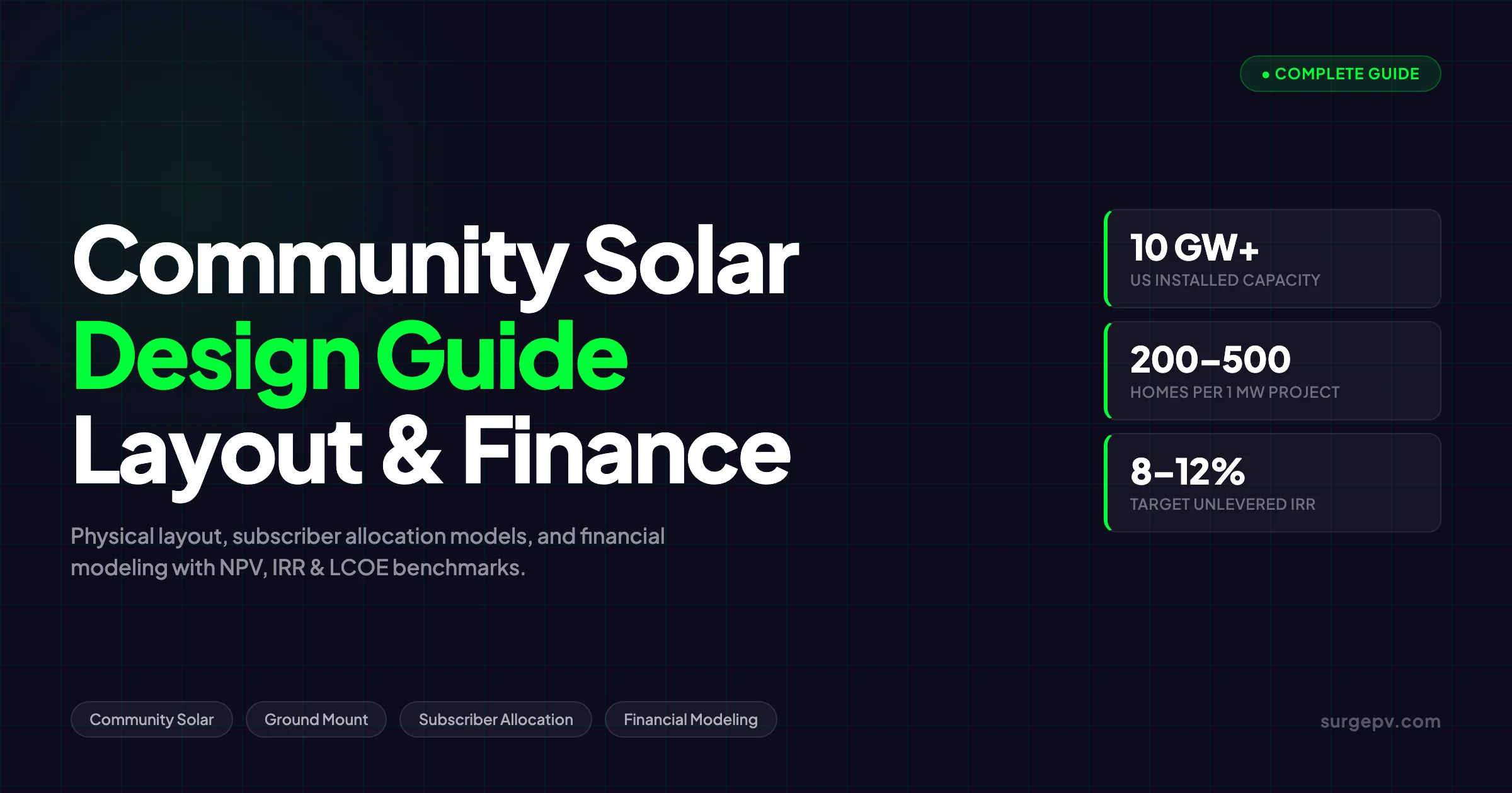
Community solar crossed 10 GW of cumulative US installed capacity in late 2025, a milestone confirmed by pv magazine in April 2026. Wood Mackenzie projects the US market will reach 14 GWdc by 2028, with new state programs in Ohio, Iowa, Michigan, and Pennsylvania driving the next growth phase. The net difference — credit received minus subscription fee — represents the subscriber's savings, typically 5–15% below retail.
Community solar crossed 10 GW of cumulative US installed capacity in late 2025, a milestone confirmed by pv magazine in April 2026. A single 1–5 MW ground-mount installation can serve 200 to 500 residential subscribers through utility bill credits, making solar accessible to renters, shaded properties, and households that cannot justify a rooftop system. Wood Mackenzie projects the US market will reach 14 GWdc by 2028, with new state programs in Ohio, Iowa, Michigan, and Pennsylvania driving the next growth phase. Also see: Us Residential Solar Market Trends 2026. For more on this topic, see Community Solar Business Model.
Community solar crossed 10 GW of cumulative US installed capacity in late 2025, a milestone confirmed by pv magazine in April 2026. Wood Mackenzie projects the US market will reach 14 GWdc by 2028, with new state programs in Ohio, Iowa, Michigan, and Pennsylvania driving the next growth phase.
Designing a community solar project is not simply building a ground-mount array and enrolling customers. It requires three separate disciplines working in parallel: physical layout design that maximizes generation on a constrained site, subscriber allocation that matches output to customer load profiles, and financial modeling that confirms the project pencils out across a 20-to-25-year operating life. This guide covers all three in the order a project team encounters them.
TL;DR — Community Solar Design
Community solar projects are typically 1–5 MW ground-mount arrays with 200–500 subscribers receiving bill credits. Physical design targets GCR of 0.30–0.45 and row spacing 3–5× panel height. Subscriber allocation is sized to 90–110% of annual load; state caps prevent any single subscriber from holding more than 40% of capacity. Financial models target 8–12% unlevered IRR with project LCOE of $30–$50/MWh and installed costs of $1.00–$1.40/W after ITC.
What Is Community Solar? Structure, Actors, and How Bill Credits Work
Community solar — also called shared solar, solar gardens, or virtual net metering — is any solar facility where generation benefits flow to multiple off-site customers. The Department of Energy defines it as “any solar project or purchasing program, within a geographic area, in which the benefits flow to multiple customers such as individuals, businesses, nonprofits, and other groups.”
Three actors define every community solar transaction:
The host is the landowner where the array is sited — often a farmer, a municipality, or a brownfield owner who leases the land to the developer.
The sponsor (developer/operator) builds, owns, and operates the project. The sponsor manages subscriber enrollment, billing relationships, and the interconnection agreement with the utility.
The subscribers pay for a share of the project’s output and receive bill credits equal to the value of their allocated generation. They do not own hardware; they own a contractual right to a portion of the electrons.
How bill credits flow:
- The array generates AC power and delivers it to the distribution grid at the point of interconnection.
- The utility measures total generation each month.
- Each subscriber’s account is credited at a per-kWh rate defined by the state program — usually the retail rate, a virtual net metering rate, or a value-of-solar tariff.
- The subscriber pays the developer a monthly fee (per kW subscribed or per kWh allocated).
- The net difference — credit received minus subscription fee — represents the subscriber’s savings, typically 5–15% below retail.
Project types by ownership structure:
| Structure | Description | Common in |
|---|---|---|
| Utility-owned | Utility builds and operates; subscribers enroll via tariff | Cooperative utilities, rural markets |
| Developer-owned SPV | Developer holds project in LLC/SPV; subscribers sign 20-year agreements | Most commercial programs |
| Nonprofit cooperative | Members co-own the LLC; subscription = equity share | Community-led projects in Germany, select US markets |
| Municipal PPA | City contracts with developer; credits distributed to municipal accounts | Anchor subscriber models |
The developer-owned SPV model dominates US commercial markets. It separates project liability from the developer’s balance sheet and allows tax equity investors to hold the ITC.
Nearly 50% of US households cannot install rooftop solar due to renting, shading, structural limitations, or affordability — which is why community solar programs exist in 44+ states and DC, with 24 jurisdictions having passed enabling legislation.
Site Selection and Physical Layout Design
Site selection drives every downstream design decision. Community solar projects are constrained by state capacity caps, distribution-level interconnection, and the need to stay within the service territory of subscribing customers’ utility accounts.
Capacity range: Most state programs cap individual projects at 1–5 MW AC. Minnesota and Colorado cap at 1 MW per project; Maine and Illinois allow up to 5 MW. Projects below 500 kW rarely pencil out after fixed development and administration costs.
Site criteria:
| Criterion | Target | Notes |
|---|---|---|
| Land area | 4–7 acres per MW | Includes access roads, setbacks, inverter pads |
| Solar resource (GHI) | Above 4.0 kWh/m²/day | NREL NSRDB or Solargis data |
| Distance to interconnection point | Under 1 mile preferred | Every extra mile adds $50,000–$150,000 in line extension costs |
| Land slope | Below 5° preferred; 15° maximum | Steeper slopes require adjustable racking and terracing |
| Shading obstructions | Minimal within 200m north | Treelines, structures, adjacent buildings |
| Zoning | Agricultural (A-1, A-2) or light industrial | Check local solar-on-farmland ordinances |
| Grid hosting capacity | Available at POI candidate | Request a Distribution Hosting Capacity Map before signing a lease |
Shading analysis is the first technical step. Before any layout is drawn, a horizon obstruction model must identify where shading losses occur across the year. Trees north of the array, adjacent structures, and topographic features all affect annual yield. A site with 5% additional shading losses relative to a clean site can reduce IRR by 1–2 percentage points over a 25-year operating period.
Use solar shadow analysis software to model horizon obstructions from aerial imagery before committing to the site. An hour of analysis can prevent months of development on an unbankable site.
Orientation and tilt for fixed-tilt ground-mount arrays in the continental US:
- Azimuth: 180° true south for maximum annual output. Deviations of ±15° lose less than 2% of annual yield.
- Tilt angle: Approximately 0.87× site latitude for maximum annual generation. At 40°N latitude, optimal fixed tilt is approximately 35°.
- Exception: If the utility has a time-of-use rate structure rewarding afternoon peak production, a 5–10° westward tilt (185–190° azimuth) can increase revenue even at a small production penalty.
Array Layout: Sizing, Strings, Row Spacing, and Ground Coverage
With tilt and orientation set, the array layout defines how panels and strings are arranged across the site.
Ground Coverage Ratio (GCR):
GCR is the ratio of panel area to total ground area. Higher GCR means more panels per acre but more inter-row shading. Community solar projects typically run GCR of 0.30–0.45.
GCR = Module Width / Row Pitch| GCR | Row Pitch | Annual Shading Loss | Best For |
|---|---|---|---|
| 0.25 | Very wide | Below 1% | High-latitude sites above 45°N |
| 0.30 | Wide | 1–2% | Moderate latitudes, conservative design |
| 0.40 | Medium | 2–4% | Typical US community solar |
| 0.50 | Narrow | 5–8% | Low-latitude sites only |
Row spacing calculation:
The minimum row pitch to avoid inter-row shading at the winter solstice solar noon:
Row Pitch = Panel Height × cos(tilt) + Panel Height × sin(tilt) / tan(sun elevation angle)At 40°N latitude with a 35° tilt and 2m panel height, minimum row pitch to avoid inter-row shading at 9am/3pm on December 21 is approximately 5.8m. Most US community solar designs target 6–7m row pitch for a GCR of approximately 0.35.
String design:
Community solar arrays almost exclusively interconnect via string inverters in combiner configurations. Key sizing rules:
- String voltage must stay within the inverter’s MPPT window (typically 500–800V DC) across the full temperature range at the site.
- String length = inverter MPPT minimum voltage ÷ (module Voc at STC × temperature correction for highest expected ambient temperature).
- For bifacial modules — standard in new projects — apply a bifacial gain factor of 5–12% depending on ground albedo (gravel: 0.25; grass: 0.20; white membrane: 0.50).
Module selection:
Community solar projects do not need the highest-efficiency modules on the market — they need the best kWh/$ over 25 years. TOPCon and PERC modules in the 440–580W range dominate new projects in 2026. A 1 MW project requires approximately 1,700–2,300 modules depending on module wattage.
Racking system:
Fixed-tilt ground-mount racking accounts for $0.10–$0.15/W of installed cost. Single-axis trackers add $0.05–$0.12/W but increase annual generation by 15–25%. For community solar, trackers are financially justified in sunbelt states (Arizona, Texas, California) where the production gain exceeds the additional capex and O&M cost.
For a detailed walkthrough of ground-mount layout design principles, see the ground-mount solar design guide.
Alternative layout configurations:
Community solar is not limited to open-field ground-mount arrays. Three alternative configurations are gaining traction in 2026:
Agrivoltaic (dual-use) layouts co-locate solar panels and agricultural operations on the same land. Panels are mounted at 8–12 feet clearance to allow crop cultivation or grazing underneath. Agrivoltaic community solar commands higher land rents (landowners receive both lease income and continued agricultural revenue) and qualifies for the Low-Income Community ITC adder in some states when sited on qualified farmland. Row spacing is wider than standard (GCR 0.20–0.30) to allow tractor access and sufficient light for crops. For design principles, see agrivoltaics design.
Canopy and carport structures allow community solar on parking lots, warehouses, or commercial rooftops. Installed cost is 30–60% higher than ground-mount due to the structural requirements, but no land acquisition is needed and urban siting keeps the project within dense subscriber populations. Canopy projects are common in New Jersey, Massachusetts, and California. For more on this topic, see Commercial Solar Carport Design Guide.
Floating solar on reservoirs, water treatment ponds, or irrigation channels eliminates land cost entirely and benefits from water cooling that improves panel efficiency by 5–10% relative to ground-mount. For a detailed treatment of floating solar project design, see floating solar farms and clean energy.
Collector system:
The collector system — cables, combiner boxes, and AC switchgear aggregating generation from individual inverters to the point of interconnection — is sized for the project’s AC output plus a 10–15% margin for future degradation. The point of interconnection (POI) is where the utility meters delivered generation for bill credit calculations.
Subscriber Allocation: Structuring the Customer Side
Physical design determines total available generation. Subscriber allocation determines who gets how much of it.
The fundamental constraint: The sum of all subscriber allocations must equal the project’s nameplate capacity. Oversubscription beyond 110% creates regulatory risk in most state programs; undersubscription means unallocated generation that earns only wholesale rates.
Two allocation methods dominate:
1. Fixed kW allocation
Each subscriber receives a fixed block of capacity (e.g., 3 kW, 5 kW, 10 kW). Bill credits are proportional to that block’s share of total generation:
Subscriber Monthly Credit = (Subscriber kW / Total Project kW) × Monthly Generation (kWh) × Retail Rate ($/kWh)Fixed allocation is simple to administer and predictable for the subscriber. The weakness: a subscriber who moves or reduces consumption still pays for their allocated capacity.
2. Bill-matched (load-sized) allocation
The subscription is sized to cover a target percentage (typically 90–110%) of the subscriber’s annual electricity consumption:
Subscription Size (kW) = Annual Load (kWh/year) / (System CF × 8,760 hours)Where System CF is the project’s annual capacity factor (typically 0.18–0.24 for fixed-tilt US sites).
Example: A residential subscriber using 9,000 kWh/year on a project with 0.20 CF:
Subscription Size = 9,000 / (0.20 × 8,760) = 5.14 kWBill-matched allocation maximizes savings for subscribers and reduces oversubscription risk. It requires annual load history from each subscriber — usually provided via an authorization to release utility data.
LMI subscriber requirements:
State programs increasingly mandate a percentage of project capacity be reserved for low-to-moderate income (LMI) subscribers:
| State | LMI Requirement | Notes |
|---|---|---|
| Colorado (2026+) | 51% of capacity | Projects approved after January 1, 2026 |
| New York | 20–30% LMI carveout | Consolidated Edison service territory |
| Illinois | 25% LMI | Community Renewable Energy Act |
| Maryland | 30% LMI | Community Solar Pilot Program |
| Massachusetts | 30% LMI | SMART program adder |
LMI subscribers typically pay lower subscription fees funded by cross-subsidies from market-rate subscribers or state grant programs. This affects revenue modeling — the financial model must explicitly account for the blended subscriber rate across both tiers.
Subscriber caps:
Most programs cap any single subscriber at 40% of the project’s total capacity. A 1 MW project cannot have any single commercial or industrial subscriber holding more than 400 kW.
Subscriber churn and reserve capacity:
Subscriber contracts are typically 20 years for commercial subscribers and 5–20 years for residential. Still, churn occurs. Most developers maintain a 10–15% waitlist buffer to backfill churned subscriptions quickly. State programs often require a replacement subscriber plan as part of the interconnection application.
Pro Tip
Sign anchor commercial subscribers — schools, municipalities, nonprofits — before launching residential enrollment. An anchor holding 20–30% of project capacity reduces subscriber acquisition cost and provides revenue certainty that improves project financing terms.
Interconnection and Grid Integration
Interconnection is the single biggest source of schedule risk in community solar development. A project that finishes construction in 12 months can wait 6–18 months for a utility interconnection study and approval.
Distribution vs. transmission interconnection:
Community solar projects (1–5 MW) interconnect at the distribution level (4–35 kV primary distribution lines), not transmission. Distribution interconnection is faster and cheaper than transmission but subject to hosting capacity constraints at the substation and feeder level.
The interconnection queue process:
- Feasibility Study — Utility confirms the POI can host the project. Timeline: 2–4 months; study cost: $5,000–$20,000.
- Impact Study — Detailed power flow and protection analysis. Timeline: 3–6 months; cost: $15,000–$50,000.
- Facilities Study — Identifies required grid upgrades. Timeline: 2–4 months; upgrade costs can reach $200,000+.
- Interconnection Agreement — Executed with the utility; defines metering, billing, and operations requirements.
Reducing interconnection risk:
- Request a Distribution Hosting Capacity Map before site selection. Areas with high hosting capacity have faster queue times and lower study costs.
- Design for a 90% AC:DC ratio (clipping ratio) to keep the AC interconnection size small, reducing upgrade requirements.
- Prioritize sites near existing distribution substations with spare transformer capacity.
Metering configuration:
Community solar projects use a single production meter at the POI. The utility reads total monthly generation and applies that figure to subscriber accounts via virtual net metering (VNM) or a community solar tariff. Individual subscribers do not need smart meters — standard interval meters suffice in most programs.
Design Your Community Solar Project in SurgePV
From site layout and shading analysis to string design and financial modeling — all in one cloud platform used across 50+ countries.
Book a DemoNo commitment required · 20 minutes · Live project walkthrough
For a direct comparison, see Arka 360 vs SurgePV.
Community Solar Financial Modeling: The Numbers That Matter
Financial modeling for community solar has more moving parts than a typical behind-the-meter commercial PV project. Revenue depends on subscriber enrollment rates, state-mandated tariff structures, and annual degradation. Costs include standard PV project costs plus subscriber management, billing platforms, and regulatory compliance — line items that do not exist in rooftop commercial projects.
Capital cost structure (2026 benchmarks):
| Cost Component | $/W DC | Share of Total |
|---|---|---|
| Modules | $0.22–$0.30 | 20–24% |
| Racking and mounting | $0.10–$0.15 | 9–12% |
| Inverters | $0.08–$0.12 | 7–10% |
| Electrical BOS (wiring, combiners, switchgear) | $0.12–$0.18 | 11–14% |
| Installation labor | $0.15–$0.22 | 13–17% |
| EPC overhead | $0.05–$0.08 | 4–6% |
| Interconnection (study + facilities upgrade) | $0.03–$0.15 | 3–12% |
| Development costs (permits, legal, land option) | $0.05–$0.10 | 4–8% |
| Contingency (10%) | $0.08–$0.12 | 7–9% |
| Total installed cost | $1.00–$1.40 | 100% |
A 1 MW DC project at the midpoint ($1.20/W) costs $1.2M before ITC. The federal Investment Tax Credit at 30% base rate reduces the tax equity basis by $360,000, bringing the net cost to approximately $840,000 before IRA adders.
Operating cost structure:
| O&M Component | Annual Cost (1 MW project) | $/kW/year |
|---|---|---|
| Module cleaning and inspection | $3,000–$6,000 | $3–$6 |
| Vegetation management | $2,000–$5,000 | $2–$5 |
| Inverter maintenance and insurance | $3,000–$8,000 | $3–$8 |
| Subscriber management and billing platform | $5,000–$15,000 | $5–$15 |
| Land lease | $3,000–$12,000 | $3–$12 |
| Insurance (property + liability) | $2,000–$5,000 | $2–$5 |
| Total annual O&M | $18,000–$51,000 | $18–$51 |
Subscriber management is a community solar-specific cost absent from behind-the-meter commercial projects. At $5–$15/kW/year, it is material. A 1 MW project with 300 subscribers costs $15–$50 per subscriber per year just for billing and customer support.
Revenue model:
Revenue comes from three sources:
1. Subscriber payments — the primary revenue stream:
Annual Subscriber Revenue = Σ (Subscriber kW × CF × 8,760 × Subscriber Rate $/kWh)2. REC sales — 1 REC generated per MWh. In high-REC-price markets (Massachusetts: $250–$380/MWh; New York: $20–$80/MWh), REC revenue adds $0.02–$0.04/kWh to effective revenue.
3. ITC and bonus depreciation — a one-time capital event that reduces net project cost by 30–70% depending on IRA adders.
Sample financial model — 1 MW DC community solar, Colorado, 2026:
| Metric | Value |
|---|---|
| System size | 1,000 kW DC / 900 kW AC |
| Installed cost | $1,200,000 |
| Annual generation (Year 1) | 1,750,000 kWh |
| Capacity factor | 19.8% |
| Subscriber rate | $0.085/kWh |
| Annual subscriber revenue (Year 1) | $148,750 |
| Annual REC revenue | $35,000 |
| Total annual revenue (Year 1) | $183,750 |
| Annual O&M | $30,000 |
| Land lease | $8,000 |
| Subscriber management | $12,000 |
| Annual EBITDA | $133,750 |
| Debt service (65% LTV, 5.5%, 20yr) | $75,000 |
| Annual cash flow to equity | $58,750 |
| ITC benefit (30% × $1.2M) | $360,000 |
| Net project cost post-ITC | $840,000 |
| Simple payback (equity) | Approximately 8.7 years |
| Unlevered IRR (25-year) | 9.4% |
| LCOE | Approximately $38/MWh |
The unlevered IRR target for community solar is 8–12%. Projects below 8% struggle to attract tax equity. Projects above 12% typically reflect favorable REC markets or low interconnection costs. Leverage (project debt) typically brings equity IRR to 12–18% depending on terms.
For a detailed walkthrough of NPV and IRR calculations for solar projects, see the solar NPV, IRR, and payback guide.
Sensitivity analysis — what moves the model most:
| Variable | ±10% Change | IRR Impact |
|---|---|---|
| Subscriber rate | ±10% | ±1.5–2.0 percentage points |
| Subscriber fill rate (enrollment speed) | ±10% | ±1.0–1.5 percentage points |
| Installed cost | ±10% | ±0.8–1.2 percentage points |
| Capacity factor / solar resource | ±10% | ±1.0–1.5 percentage points |
| O&M cost escalation | ±10% | ±0.3–0.5 percentage points |
Subscriber fill rate is the most overlooked risk in community solar financial modeling. A project that takes 18 months to reach full subscription instead of 6 months loses over a year of full revenue while still incurring full O&M, debt service, and land lease costs. Model this explicitly in the base case — do not assume Day 1 full enrollment.
Revenue Structures and Pricing Models
Setting the subscriber rate is the most consequential financial decision in community solar development. The rate must satisfy three constraints simultaneously:
- Savings constraint: The subscriber must pay less than their current retail rate — typically 5–15% less to drive enrollment.
- Revenue constraint: The rate must cover O&M, debt service, and deliver adequate equity yield.
- Regulatory constraint: Many state programs set maximum and minimum subscriber rates, sometimes pegged to a percentage of the retail rate.
Three common pricing structures:
Fixed per-kWh rate: Subscriber pays a fixed $/kWh for all energy allocated to their account (e.g., $0.085/kWh vs. $0.115/kWh retail). Simple, transparent, easy to model. Risk: if retail rates fall, subscriber savings disappear and churn increases.
Indexed rate (% of retail): Subscriber rate is set at 88–92% of the retail rate, adjusted annually. Guarantees the subscriber a savings percentage regardless of retail rate movements. More complex to administer but reduces churn risk.
Fixed monthly subscription fee: Subscriber pays a flat monthly fee per kW subscribed (e.g., $6.50/kW/month). Revenue is predictable for the developer regardless of solar generation. Risk: in low-production months, the subscriber may receive fewer bill credits than their fixed fee — creating dissatisfaction.
Pricing Recommendation
For new 2026 projects, the indexed rate (85–90% of retail) with a 3–5% annual escalator cap provides the best balance of subscriber retention and revenue predictability. It guarantees the subscriber a floor savings and lets the developer participate in retail rate increases over time.
Commercial vs. residential pricing:
Commercial subscribers (C&I accounts) typically negotiate lower rates due to larger subscription blocks (50–400 kW per account). A single commercial subscriber at $0.075/kWh on 200 kW provides more predictable revenue than 40 residential subscribers at $0.085/kWh on 5 kW each — but the commercial discount erodes project revenue by 6–12%.
Tax Credits and IRA Adders
The Inflation Reduction Act (IRA) extended and expanded the ITC through at least 2032. The base rate is 30%, with stackable adders that can bring the effective credit to 50–70% for qualifying projects.
IRA adder summary for community solar:
| Adder | Bonus Rate | Qualifying Condition |
|---|---|---|
| Base ITC | 30% | Projects above 1 MW meeting prevailing wage and apprenticeship requirements |
| Energy Community | +10% | Site in a coal closure area or area with fossil fuel employment above 0.17% |
| Low-Income Community | +10–20% | Sited in a census tract with median income at or below 80% of area median |
| Domestic Content | +10% | 40%+ of steel, iron, and manufactured components made in the US |
| Maximum combined | 60–70% | Projects qualifying for all applicable adders |
For community solar specifically, the Low-Income Bonus Credit at 20% is available for projects sited in qualified census tracts — not only for the LMI subscriber carveout. A project qualifying for base + Energy Community + Low-Income adder receives a 50% ITC. On a $1.2M project, that is $600,000 in federal tax credits.
Bonus depreciation:
Under current IRA provisions, 60% bonus depreciation applies to community solar assets placed in service in 2026, stepping down to 40% in 2027. Combined with MACRS 5-year depreciation for the remaining basis, developers or tax equity investors recover most of the capital cost in Years 1–2.
For the complete US solar tax credit landscape including ITC mechanics and IRA adder stacking rules, see the solar IRA tax credits US guide.
Legal and Business Structure
Most commercial community solar projects are structured as a Special Purpose Vehicle (SPV) — typically a single-member or multi-member LLC that holds the project assets, interconnection agreement, and subscriber contracts.
Typical legal entity stack:
Developer Entity (HoldCo)
    └── Project LLC (SPV)
            ├── Real Property: Land Lease Agreement
            ├── Revenue: Subscriber Contracts + Utility VNM Agreement
            ├── Financing: Construction Loan → Term Debt + Tax Equity
            └── Operations: O&M Agreement
Key contracts in a community solar deal:
Land Lease Agreement — 25–35 year term. Rent typically $500–$1,500/acre/year, sometimes with a production-linked escalator.
Interconnection Agreement — Executed with the utility. Defines metering configuration, protection requirements, and any facilities upgrade cost recovery.
Subscriber Contracts — Residential: 5–20 years with transfer rights if subscriber moves within service territory. Commercial: 10–25 years.
Community Solar Tariff Agreement — In regulated markets, the utility’s tariff governs the credit rate. In deregulated markets, the developer negotiates a VNM or net billing agreement directly.
O&M Agreement — If the developer outsources operations, the O&M provider typically charges $15–$25/kW/year on a fixed-fee basis.
State Program Requirements: The Regulatory Landscape
No two state community solar programs are the same. Capacity, subscriber mix, contract terms, and billing structure must all comply with state-specific rules.
Key program parameters by state (2026):
| State | Max Project Size | Min Subscribers | LMI Requirement | Credit Rate | Status |
|---|---|---|---|---|---|
| Minnesota | 1 MW | 5 | None (voluntary) | Retail rate | Active — market mature |
| New York | 5 MW | 10 | 20–30% | Value of DER rate | Active — queues open |
| Illinois | 2 MW | 2 | 25% | Retail rate | Active — CREA program |
| Colorado | 2 MW | 10 | 51% (2026+ projects) | Retail rate | Active — Xcel and co-ops |
| Massachusetts | 2 MW | 10 | 30% | SMART adder rate | Active |
| Maryland | 2 MW | 10 | 30% | Retail rate | Active — Pilot program |
| Maine | 5 MW | None | 10% | Retail rate | Active |
| California | 3 MW | None | SOMAH program only | NEM rate | SOMAH active |
| Ohio | 5 MW | TBD | TBD | TBD | New program — rules pending 2026 |
| Michigan | 3 MW | TBD | TBD | TBD | New program — rules pending 2026 |
Interconnection timeline by state:
| State | Average Timeline | Key Bottleneck |
|---|---|---|
| New York | 12–24 months | Con Edison queue backlog |
| Illinois | 6–12 months | Ameren and ComEd study times |
| Colorado | 8–16 months | Xcel capacity constraint in Front Range |
| Massachusetts | 6–10 months | Eversource and National Grid |
| Minnesota | 4–8 months | Xcel and Cooperative queues |
For European community solar markets, the policy landscape operates under distinct EU renewable energy directives. Germany’s Mieterstrom and Gemeinschaftliche Gebäudeversorgung models differ structurally from US VNM programs. See community solar projects in Germany for a full breakdown of the German framework, including the Solarpaket I reforms. Also see: European Solar Incentives. For Europe-specific compliance details, see Europe solar compliance.
Using Solar Design Software for Community Solar Projects
Community solar projects require more design complexity than a typical commercial rooftop installation. A project team needs to:
- Model the site in 3D with topography and horizon obstructions
- Calculate row spacing and GCR for the specific latitude and module dimensions
- Run shading analysis at winter solstice conditions across every row
- Size the inverter array with appropriate clipping ratios
- Generate a single-line diagram and BOM for the interconnection application
- Model generation at P50 and P90 probability levels for lender bankability
Solar design software that integrates layout, shading, and financial modeling eliminates manual errors from passing data between separate tools. SurgePV’s cloud-based platform handles site layout, shadow analysis, generation modeling, and the generation and financial tool in a single workflow — generating P50/P90 yield estimates and preliminary financial outputs from the same project file.
P50 and P90 yield modeling for lender bankability:
Lenders and tax equity investors require a bankable energy yield assessment before closing project financing. This means modeling generation at two probability levels:
- P50 — the median expected annual generation (50% probability of exceedance). Used for base-case revenue projections.
- P90 — the conservative yield (90% probability of exceedance, meaning only a 10% chance of falling below this number). Used for debt service coverage calculations; lenders typically size the loan so that P90 generation is sufficient to cover debt payments.
The difference between P50 and P90 on a fixed-tilt US ground-mount project is typically 8–15%, reflecting inter-annual solar resource variability. A project modeled at P50 of 1,750,000 kWh/year might have a P90 of 1,530,000 kWh/year. Lenders will underwrite debt coverage against the P90 figure — so the financial model must run separately at both probability levels.
Third-party energy yield assessments from firms like DNV, UL, or kWh Analytics are required by most lenders for projects above $5M total cost. For smaller projects, a certified report generated directly from a bankable solar design platform can substitute, saving $15,000–$40,000 in consultant fees.
For lender review, the ability to export a bankable energy yield report directly from the design tool removes a costly third-party modeling step. The commercial solar design software buyer guide compares platforms suited to community solar scale if you are evaluating options.
Solar proposal software is also relevant at the subscriber enrollment stage. Per-subscriber savings illustrations generated from the project’s yield model close subscriptions faster and reduce churn by setting accurate savings expectations upfront.
Step-by-Step: From Concept to Commercial Operation
A community solar project moves through eight phases from initial concept to first bill credits.
Phase 1: Site Identification and Feasibility (1–3 months)
Screen sites for solar resource, interconnection proximity, and state program eligibility. Pull utility hosting capacity maps. Confirm the POI candidate has available capacity. Secure a site control option — not a full lease, just the right to negotiate exclusivity for 6–12 months. Run a preliminary financial model using NREL’s System Advisor Model (SAM) community solar financial model for yield and a simplified cost estimate.
Phase 2: Interconnection Application (1–2 months)
Submit the interconnection application to the utility with a preliminary single-line diagram. Pay the study deposit ($5,000–$20,000). This step starts the queue clock — earlier is better, even if the project design changes later. The queue position is preserved as long as the application remains active.
Phase 3: Detailed Engineering and Layout Design (2–4 months)
Commission a topographic survey and geotechnical study. Run detailed shading analysis with a 3D terrain model. Complete the array layout: module count, string configuration, inverter selection, collector system. Generate the full engineering package: site plan, electrical single-line, grounding plan, BOM.
Phase 4: Permitting (2–6 months)
Building permits from the local AHJ. Stormwater and erosion control plan. State program capacity reservation application. Environmental permits if required by site history (contaminated land, wetlands adjacency).
Phase 5: Financing Close (3–6 months)
Complete financial model with bankable P50 energy yield from the engineering package. Negotiate construction loan and term debt with a lender. Bring in a tax equity investor for ITC monetization. Execute land lease, interconnection agreement, and subscriber management platform agreement.
Phase 6: Subscriber Enrollment (3–12 months, can overlap Phase 5)
Launch marketing for subscriber enrollment via digital, direct mail, and anchor subscriber outreach. Execute subscriber contracts as enrollment builds toward 90–100% of capacity. Confirm LMI subscriber participation meets state program requirements.
Phase 7: Construction (3–6 months)
EPC contractor mobilizes following Notice to Proceed from the lender. Pile driving, racking, module installation, electrical work. Utility witness testing and interconnection energization.
Phase 8: Commercial Operation (COD)
Utility activates VNM tariff or community solar tariff for all subscribers. Bill credits begin flowing to subscriber accounts. Developer submits ITC certification and claim. O&M contract activates.
Total timeline from site identification to COD: 18–36 months in most US markets, with interconnection queue wait time as the primary variable.
Conclusion
Community solar project design requires three disciplines to converge on a single bankable plan. Physical layout follows established ground-mount engineering principles with GCR, row spacing, and string configuration optimized for the specific site and latitude. Subscriber allocation adds a business model layer: matching generation to customer load profiles, meeting state LMI mandates, and managing churn risk. Financial modeling ties it together with a 25-year cash flow projection that must satisfy both lender debt service coverage and equity return requirements.
Three action items for development teams starting a community solar project now:
- Start the interconnection application before the design is final. Queue time is the longest single delay; an early application preserves your position even if the design evolves.
- Sign anchor commercial subscribers first. A 20–30% anchor subscription from a municipality or commercial tenant reduces financing risk and subscriber acquisition cost.
- Model the LMI requirement impact on IRR before committing to a state program. A 51% LMI carveout with discounted subscriber rates reduces revenue by 10–20% — verify the financial model accounts for this before signing a land lease.
Frequently Asked Questions
What is community solar and how does it work?
Community solar is a shared solar facility where multiple subscribers receive bill credits proportional to their share of the project’s output. The array is built at a single site, energy flows to the grid, and each subscriber’s utility bill reflects their allocated generation — no rooftop panels required.
How do you design a community solar project layout?
Community solar layout design starts with site selection (1–5 MW typical capacity), followed by shading analysis, optimal tilt and row spacing calculations, inverter sizing, and interconnection planning. The physical design follows ground-mount solar principles but is constrained by state capacity caps and subscriber count targets.
What is subscriber allocation in community solar?
Subscriber allocation assigns each participant a defined percentage of the project’s output. Allocation can be fixed (e.g., 5 kW per subscriber) or bill-matched (sized to cover each subscriber’s annual load). Most state programs cap any single subscriber at 40% of total capacity.
How is community solar financially modeled?
Community solar financial modeling projects revenue from subscriber payments against capital costs (typically $1.00–$1.40/W installed), O&M, interconnection fees, and debt service. Key outputs are NPV, IRR (target 8–12% unlevered), LCOE, and payback period.
How many subscribers does a community solar project need?
A 1 MW community solar project typically supports 200–500 residential subscribers depending on local electricity rates and subscription sizing. Most programs require a minimum of 10 subscribers; practical viability often requires 50+ to justify marketing and billing infrastructure costs.
What is the minimum size for a community solar project?
Most state programs set a minimum capacity of 100 kW and a maximum of 1–5 MW per project, though some states allow up to 20 MW. The practical minimum for financial viability is typically 500 kW due to fixed development, interconnection, and administration costs.
How do community solar projects make money?
Revenue comes from subscriber payments — either a fixed monthly fee per kW subscribed or a per-kWh rate. Developers also earn from federal tax credits (ITC), REC sales, and in some states, utility capacity payments.
What states have community solar programs?
As of 2026, 24 states plus DC have enacted community solar enabling legislation. The most active markets are Minnesota, New York, Illinois, Colorado, Massachusetts, and Maryland. New programs in Ohio, Iowa, Michigan, and Pennsylvania are expected to drive the next growth wave.