Quick Answer
A developer in Rajasthan once leased 80 hectares for what he calculated as a 50 MWp fixed-tilt plant. After geotechnical surveys, setback compliance, and access road routing, the usable module area shrank to 52 hectares. The PPA was already signed at 50 MWp. This guide is a practical solar land area calculator.
Ground-mount solar projects live or die on land math. A developer in Rajasthan once leased 80 hectares for what he calculated as a 50 MWp fixed-tilt plant. After geotechnical surveys, setback compliance, and access road routing, the usable module area shrank to 52 hectares. The project dropped to 32 MWp. The PPA was already signed at 50 MWp. That story is more common than most developers admit. Also see: Us Residential Solar Market Trends 2026.
A developer in Rajasthan once leased 80 hectares for what he calculated as a 50 MWp fixed-tilt plant. After geotechnical surveys, setback compliance, and access road routing, the usable module area shrank to 52 hectares. The PPA was already signed at 50 MWp.
This guide is a practical solar land area calculator. It covers how to estimate hectares per MWp for any project size, how module efficiency and row spacing change the numbers, what access roads and substations add, and where standard estimates fall short. Every table uses real-world data from NREL, IEA-PVPS, and operational projects. All figures are current as of 2026.
TL;DR — Solar Land Area Calculator
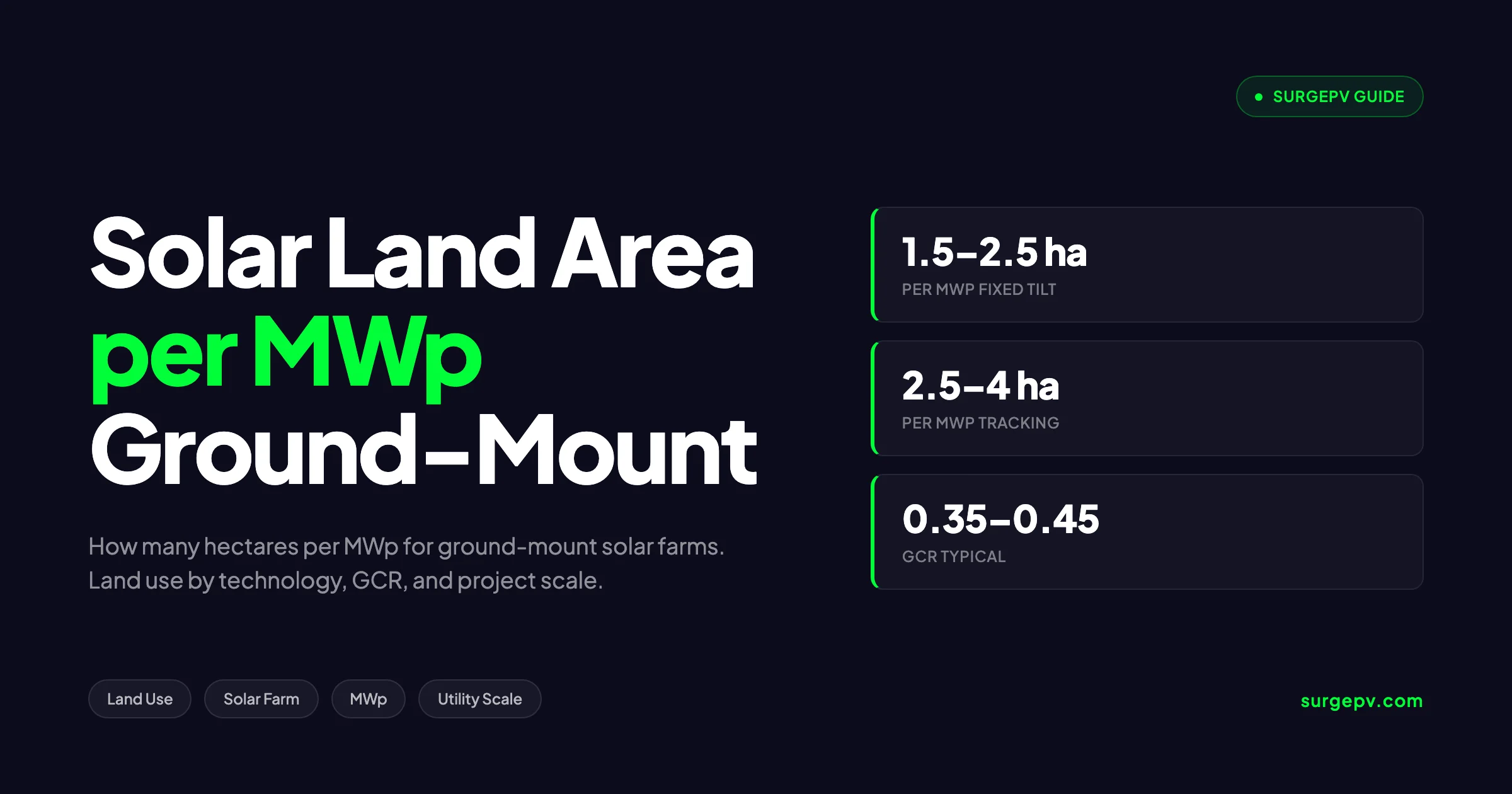
A fixed-tilt solar farm needs 1.5 to 2.5 hectares per MWp depending on module efficiency and row spacing. Single-axis tracking needs 2.2 to 2.8 hectares per MWp. High-efficiency modules (over 22%) reduce land use by 15 to 25%. Add 10 to 20% for roads, substations, and setbacks.
In this guide:
- How solar land area calculators work — inputs, formulas, and limits
- Typical land use per MWp: utility scale vs. commercial ground-mount
- Module efficiency impact on land area
- Row spacing, tilt angle, and ground coverage ratio explained
- Access roads, substations, and buffer zones — the hidden 20%
- Land area by project type: fixed tilt, single-axis tracking, agrivoltaics
- Land area tables by MWp size: 1 MW, 5 MW, 10 MW, 50 MW, 100 MW
- Land use efficiency: MWp per hectare by technology
- Environmental and zoning considerations
- Agrivoltaics: dual land use and area requirements
- When land area estimates are misleading — what most developers get wrong
- Real project land use examples
How Solar Land Area Calculators Work
A solar land area calculator estimates the physical footprint of a ground-mount PV project. It takes project parameters and returns a land requirement in hectares or acres. Most calculators follow the same basic logic.
Core Inputs
| Input | Typical Range | Impact on Output |
|---|---|---|
| System capacity (MWp) | 0.5 to 500+ | Direct linear scaling |
| Module wattage (W) | 450 to 720 | Higher wattage = fewer modules = less land |
| Module efficiency (%) | 19 to 23 | Higher efficiency = smaller module area per Wp |
| Tilt angle (degrees) | 15 to 35 | Affects row spacing requirement |
| Row spacing factor | 2.0x to 4.5x module height | Wider spacing = more land per MWp |
| GCR target | 0.30 to 0.50 | Higher GCR = denser layout |
| Tracking type | Fixed / 1-axis / 2-axis | Trackers need wider spacing |
The Basic Formula
The calculation has three steps:
Step 1: Module area per MWp
Module area (m²) = Module wattage (W) / (1000 × Module efficiency)
Modules per MWp = 1,000,000 / Module wattage
Total module area per MWp = Modules per MWp × Module area
For a 550 W module at 21% efficiency:
- Module area = 550 / (1000 × 0.21) = 2.62 m²
- Modules per MWp = 1,000,000 / 550 = 1,818
- Total module area per MWp = 1,818 × 2.62 = 4,763 m² = 0.48 hectares
Step 2: Module field area (accounting for GCR)
Module field area = Total module area / GCRAt GCR = 0.40:
- Module field area = 0.48 / 0.40 = 1.20 hectares per MWp
Step 3: Total site area (adding infrastructure)
Total site area = Module field area × (1 + Infrastructure factor)With a 15% infrastructure factor:
- Total site area = 1.20 × 1.15 = 1.38 hectares per MWp
Calculator Limitations
No online calculator knows your site’s slope, soil type, or local setback rules. A calculator gives a starting point. The real number comes from a detailed layout using solar design software that models shading, terrain, and civil constraints. Shadow analysis software identifies shading issues before installation.
Pro Tip — Always Model the Actual Site
Flat land calculators assume uniform terrain. A 3% slope facing south can increase yield by 1 to 2% but may require stepped racking. A 5% slope facing north can reduce annual yield by 4 to 8%. Always import topographic data into your layout tool before finalizing land estimates.
Typical Land Use Per MWp: Utility Scale vs. Commercial Ground-Mount
Land use per MWp varies more than most developers expect. The same 10 MWp project can need 15 hectares or 28 hectares depending on choices made early in design.
Land Use by System Type
| System Type | Hectares per MWp | Acres per MWp | Typical GCR | Notes |
|---|---|---|---|---|
| Fixed tilt, standard modules (19–20%) | 1.8 – 2.2 | 4.5 – 5.4 | 0.35 – 0.42 | Most common utility-scale configuration |
| Fixed tilt, high-efficiency (21–23%) | 1.5 – 1.8 | 3.7 – 4.4 | 0.38 – 0.45 | Best land use for standard ground-mount |
| Single-axis tracking | 2.2 – 2.8 | 5.4 – 6.9 | 0.30 – 0.38 | Higher yield per MWp, more land per MWp |
| Dual-axis tracking | 3.0 – 4.0 | 7.4 – 9.9 | 0.22 – 0.30 | Rare at utility scale; high maintenance |
| Agrivoltaics (elevated) | 2.5 – 4.0 | 6.2 – 9.9 | 0.20 – 0.35 | Height and spacing driven by crop needs |
| Commercial rooftop (reference) | 0.08 – 0.12 | 0.2 – 0.3 | 0.60 – 0.80 | Not ground-mount; included for comparison |
Source: NREL “Land Use and Solar Energy” technical report, 2024; IEA-PVPS Task 13 survey data.
Utility-Scale vs. Commercial Ground-Mount
Utility-scale projects (50 MWp and above) achieve better land efficiency than smaller projects. Large sites allow optimized row spacing without edge effects. Access roads serve more capacity per meter. Substation cost is amortized over more megawatts. A 200 MWp project typically achieves 1.6 to 1.9 hectares per MWp with fixed-tilt high-efficiency modules.
Commercial ground-mount projects (0.5 to 5 MWp) often use land less efficiently. Small sites have more edge area relative to module area. Setbacks consume a larger percentage of total land. Access roads cannot be shared across as much capacity. A 2 MWp project on a constrained site may need 2.2 to 2.6 hectares per MWp.
Key Takeaway — Scale Matters
Utility-scale projects achieve 15 to 25% better land use efficiency per MWp than commercial-scale projects. The difference comes from shared infrastructure, optimized row spacing, and lower edge-to-area ratios. When evaluating a site, use scale-appropriate land use figures, not generic averages.
Module Efficiency Impact on Land Area
Module efficiency is the most powerful lever for reducing land use. It is also the most expensive lever — high-efficiency modules cost more per watt.
How Efficiency Changes the Math
| Module Efficiency | Typical Wattage | Module Area per MWp | Hectares per MWp (GCR 0.40) |
|---|---|---|---|
| 19.0% | 450 W | 5,263 m² | 1.32 |
| 20.0% | 500 W | 5,000 m² | 1.25 |
| 21.0% | 550 W | 4,762 m² | 1.19 |
| 22.0% | 600 W | 4,545 m² | 1.14 |
| 23.0% | 670 W | 4,348 m² | 1.09 |
Table shows module field area only. Add 10 to 20% for infrastructure.
A 2 percentage point efficiency gain (from 20% to 22%) reduces module area by 9%. On a 100 MWp project, that saves approximately 4 hectares of module field area. At a land lease rate of $500 per hectare per year, that is $2,000 in annual savings — modest, but the real value is in accessing smaller or constrained sites.
Bifacial Modules and Effective Land Use
Bifacial modules capture light on both sides. The rear-side gain depends on albedo (ground reflectivity): For more on this topic, see Bifacial Solar Panel Design Guide.
| Ground Type | Albedo | Bifacial Gain | Effective MWp per Hectare Increase |
|---|---|---|---|
| White gravel / sand | 0.50 – 0.70 | 15 – 25% | 15 – 25% |
| Grass / vegetation | 0.20 – 0.30 | 8 – 12% | 8 – 12% |
| Dark soil | 0.10 – 0.15 | 4 – 7% | 4 – 7% |
A fixed-tilt bifacial system on grass achieves the energy output of a 1.12 MWp monofacial system from a 1.00 MWp footprint. That is a 12% effective improvement in land use without changing the physical layout.
Pro Tip — Match Module to Land Cost
On expensive land ($1,000+ per hectare per year), high-efficiency modules pay for themselves through reduced lease costs. On cheap desert land ($100 per hectare per year), standard modules are usually more economical. Run the math: land savings + reduced civil work vs. module cost premium.
Row Spacing, Tilt Angle, and Ground Coverage Ratio
Row spacing and tilt angle determine how much of your land actually holds modules. These are the variables that separate a dense, efficient layout from a sprawling, expensive one.
Understanding Ground Coverage Ratio (GCR)
GCR is simple: module area divided by total land area.
GCR = Total module area / Total module field areaA GCR of 0.40 means 40% of your land is covered by modules. The other 60% is row spacing, access paths, and structural gaps.
| GCR | Layout Density | Typical Use Case |
|---|---|---|
| 0.25 – 0.30 | Very open | Single-axis tracking, high-latitude sites |
| 0.35 – 0.42 | Standard | Fixed-tilt utility scale, most common |
| 0.45 – 0.50 | Dense | Fixed-tilt commercial, land-constrained |
| 0.55 – 0.65 | Very dense | Carport, agrivoltaics with tight spacing |
Row Spacing and Sun Angle
Minimum row spacing prevents inter-row shading during peak sun hours. The standard rule: no shading between 9 AM and 3 PM on the winter solstice.
The spacing formula:
Row spacing = Module row height × Spacing factor
Module row height = Module width × sin(tilt angle)
At 35 degrees latitude with 30-degree tilt:
| Module Orientation | Module Width | Tilt | Row Height | Spacing Factor | Row Spacing |
|---|---|---|---|---|---|
| Portrait (1.13 m wide) | 1.13 m | 30° | 0.57 m | 3.0× | 1.71 m |
| Landscape (2.28 m wide) | 2.28 m | 30° | 1.14 m | 3.0× | 3.42 m |
Landscape orientation doubles row height and doubles spacing requirement. Most utility-scale projects use portrait orientation for this reason.
Tilt Angle Tradeoffs
| Tilt Angle | Annual Yield (relative) | Row Spacing Need | Land Use per MWp |
|---|---|---|---|
| 15° | 97% | Low | Lowest |
| 20° | 99% | Medium | Low |
| 25° | 100% | Medium | Standard |
| 30° | 99% | High | Higher |
| 35° | 97% | Very high | Highest |
Relative to optimal tilt at 35° latitude. Actual optimal tilt equals latitude ±5°.
The tradeoff: Higher tilt increases winter yield but requires wider row spacing. At most latitudes, the land cost of wider spacing outweighs the energy gain beyond 5 to 10 degrees above latitude-matched tilt. Flattening tilt to 20 degrees can reduce land use by 15 to 20% with only 1 to 3% energy loss.
What Most Developers Get Wrong About Tilt
Developers often design at latitude-matched tilt (30° at 30° latitude) because it maximizes annual yield per module. But it does not maximize annual yield per hectare. A flatter tilt with tighter spacing can produce more total energy from a fixed land area. When land is the constraint, optimize for kWh per hectare, not kWh per module.
Access Roads, Substations, and Buffer Zones
The module field is only part of the story. Infrastructure consumes 10 to 20% of total site area. On constrained sites, it can consume 30% or more.
Infrastructure Land Requirements
| Infrastructure Type | Area per MWp | Typical Total (100 MWp) | Notes |
|---|---|---|---|
| Internal access roads | 0.10 – 0.20 ha/MWp | 10 – 20 ha | 4–6 m wide, spaced every 200–400 m |
| Perimeter roads | 0.02 – 0.05 ha/MWp | 2 – 5 ha | Security and maintenance access |
| Substation / switchyard | 0.01 – 0.03 ha/MWp | 1 – 3 ha | Scales with voltage level |
| Inverter pads / stations | 0.01 – 0.02 ha/MWp | 1 – 2 ha | Central inverters need more space |
| Perimeter setbacks | 0.05 – 0.15 ha/MWp | 5 – 15 ha | Varies by jurisdiction |
| Drainage / detention | 0.02 – 0.05 ha/MWp | 2 – 5 ha | Required in some jurisdictions |
| Total infrastructure | 0.21 – 0.50 ha/MWp | 21 – 50 ha | 10 – 25% of module field |
Substation Sizing
The substation is the largest single non-module land user. Its size depends on the interconnection voltage:
| Project Size | Typical Voltage | Substation Area |
|---|---|---|
| 1 – 5 MWp | 11 – 33 kV | 0.1 – 0.3 ha |
| 5 – 20 MWp | 33 – 66 kV | 0.3 – 0.8 ha |
| 20 – 100 MWp | 66 – 132 kV | 0.5 – 1.5 ha |
| 100 – 500 MWp | 132 – 220 kV | 1.0 – 3.0 ha |
High-voltage substations need larger clearances for safety and arc-flash protection. A 200 MWp project at 220 kV may need a 2-hectare substation — equivalent to 1% of total land.
Setback and Buffer Requirements
Setback rules vary dramatically by country and municipality:
| Jurisdiction | Typical Road Setback | Residential Setback | Water Body Setback |
|---|---|---|---|
| United States (varies by state) | 15 – 50 m | 50 – 150 m | 30 – 100 m |
| United Kingdom | 20 – 30 m | 50 – 100 m | 50 – 100 m |
| Germany | 20 – 40 m | 100 – 200 m | 50 – 100 m |
| India | 15 – 30 m | 30 – 50 m | 30 – 50 m |
| Australia | 20 – 40 m | 50 – 100 m | 40 – 80 m |
These setbacks are non-negotiable. A 100-hectare rectangular site with 50-meter setbacks on all sides loses approximately 18% of gross area to buffers.
Pro Tip — Negotiate Setbacks Early
Some jurisdictions allow reduced setbacks with vegetative screening or berming. A 5-meter landscape berm can replace a 20-meter setback in certain counties. Engage local planning staff before finalizing site layouts — informal guidance often differs from published codes.
Land Area by Project Type
Different project types have fundamentally different land use profiles. Choosing the right technology for your land constraints is a critical early decision.
Fixed-Tilt Systems
Fixed-tilt is the default choice for most ground-mount projects. Modules are mounted at a fixed angle, usually facing south (northern hemisphere) or north (southern hemisphere).
Advantages: Lowest cost per MWp, simplest maintenance, highest GCR, best land use.
Disadvantages: 15 to 25% lower annual yield than tracking for the same module capacity.
Typical land use: 1.5 to 2.2 hectares per MWp (including infrastructure).
Single-Axis Tracking
Single-axis tracking (1T) rotates modules on a north-south axis to follow the sun east to west. It increases annual energy yield by 15 to 25% compared to fixed tilt.
Advantages: Higher yield per MWp, better afternoon production matching peak demand.
Disadvantages: Wider row spacing (tracker rotation clearance), higher maintenance, more land per MWp.
Typical land use: 2.2 to 2.8 hectares per MWp (including infrastructure).
The yield vs. land tradeoff: A 1T system needs 30 to 40% more land but produces 15 to 25% more energy. The net land use per MWh is roughly comparable — sometimes better, sometimes worse, depending on latitude and local pricing.
Agrivoltaics
Agrivoltaics places solar panels above active agricultural land. Panel height ranges from 2.5 meters (sheep grazing) to 5 meters (mechanized crop farming). See Agrivoltaics Design for detailed guidance.
Advantages: Dual land revenue, reduced water evaporation, crop shading in hot climates, social license.
Disadvantages: Lowest MWp per hectare, complex mounting structures, limited crop compatibility.
Typical land use: 2.5 to 4.0 hectares per MWp (including infrastructure).
France leads in agrivoltaic regulation. The French government requires minimum panel height (2.5 to 4.5 meters depending on crop), maximum ground coverage ratio (0.40 to 0.50), and proof of maintained agricultural output. Germany’s EEG 2023 introduced agri-PV tariffs with specific spacing requirements. Also see: France solar feed-in tariffs. Read more about Agricultural Solar Case Study.
Design Solar Farms with Precision
SurgePV’s solar design software models terrain, shading, and row spacing automatically. Get accurate land use estimates before you sign the lease.
Explore Solar Design SoftwareFree trial · No credit card · Import terrain data
For a direct comparison, see Arka 360 vs SurgePV.
Land Area Tables by MWp Size
These tables give practical land estimates for common project sizes. All figures include a 15% infrastructure factor.
Fixed-Tilt Systems (Standard Modules, 20% Efficiency)
| Project Size | Module Field Area | Infrastructure (15%) | Total Site Area | Acres |
|---|---|---|---|---|
| 1 MWp | 2.0 ha | 0.3 ha | 2.3 ha | 5.7 |
| 5 MWp | 10.0 ha | 1.5 ha | 11.5 ha | 28.4 |
| 10 MWp | 20.0 ha | 3.0 ha | 23.0 ha | 56.8 |
| 25 MWp | 50.0 ha | 7.5 ha | 57.5 ha | 142.1 |
| 50 MWp | 100.0 ha | 15.0 ha | 115.0 ha | 284.2 |
| 100 MWp | 200.0 ha | 30.0 ha | 230.0 ha | 568.4 |
| 200 MWp | 400.0 ha | 60.0 ha | 460.0 ha | 1,136.8 |
Fixed-Tilt Systems (High-Efficiency Modules, 22% Efficiency)
| Project Size | Module Field Area | Infrastructure (15%) | Total Site Area | Acres |
|---|---|---|---|---|
| 1 MWp | 1.7 ha | 0.3 ha | 2.0 ha | 4.9 |
| 5 MWp | 8.5 ha | 1.3 ha | 9.8 ha | 24.2 |
| 10 MWp | 17.0 ha | 2.6 ha | 19.6 ha | 48.4 |
| 25 MWp | 42.5 ha | 6.4 ha | 48.9 ha | 120.8 |
| 50 MWp | 85.0 ha | 12.8 ha | 97.8 ha | 241.6 |
| 100 MWp | 170.0 ha | 25.5 ha | 195.5 ha | 483.1 |
| 200 MWp | 340.0 ha | 51.0 ha | 391.0 ha | 966.2 |
Single-Axis Tracking Systems
| Project Size | Module Field Area | Infrastructure (15%) | Total Site Area | Acres |
|---|---|---|---|---|
| 1 MWp | 2.6 ha | 0.4 ha | 3.0 ha | 7.4 |
| 5 MWp | 13.0 ha | 2.0 ha | 15.0 ha | 37.1 |
| 10 MWp | 26.0 ha | 3.9 ha | 29.9 ha | 73.9 |
| 25 MWp | 65.0 ha | 9.8 ha | 74.8 ha | 184.8 |
| 50 MWp | 130.0 ha | 19.5 ha | 149.5 ha | 369.5 |
| 100 MWp | 260.0 ha | 39.0 ha | 299.0 ha | 739.0 |
| 200 MWp | 520.0 ha | 78.0 ha | 598.0 ha | 1,478.0 |
Agrivoltaic Systems
| Project Size | Module Field Area | Infrastructure (20%) | Total Site Area | Acres |
|---|---|---|---|---|
| 1 MWp | 3.2 ha | 0.6 ha | 3.8 ha | 9.4 |
| 5 MWp | 16.0 ha | 3.2 ha | 19.2 ha | 47.4 |
| 10 MWp | 32.0 ha | 6.4 ha | 38.4 ha | 94.9 |
| 25 MWp | 80.0 ha | 16.0 ha | 96.0 ha | 237.2 |
Agrivoltaics uses a 20% infrastructure factor due to wider access roads for farm equipment and larger structural foundations.
Key Takeaway — Use the Right Table
A 50 MWp fixed-tilt project needs 115 hectares with standard modules or 98 hectares with high-efficiency modules. That 17-hectare difference is worth $8,500 to $17,000 per year in land lease savings. Always specify module efficiency when estimating land — generic “2 hectares per MWp” rules can mislead by 20% or more.
Land Use Efficiency: MWp Per Hectare by Technology
Flipping the metric — MWp per hectare instead of hectares per MWp — makes it easier to compare technologies at a glance.
MWp per Hectare Comparison
| Technology | Modules | MWp per Hectare (Module Field) | MWp per Hectare (Total Site) |
|---|---|---|---|
| Fixed tilt, 19% efficiency | 450 W | 0.53 | 0.46 |
| Fixed tilt, 21% efficiency | 550 W | 0.63 | 0.55 |
| Fixed tilt, 23% efficiency | 670 W | 0.75 | 0.65 |
| Single-axis tracking, 21% | 550 W | 0.42 | 0.36 |
| Single-axis tracking, 23% | 670 W | 0.50 | 0.43 |
| Agrivoltaics, 21% | 550 W | 0.31 | 0.26 |
| Agrivoltaics, 23% | 670 W | 0.38 | 0.31 |
Energy Yield Per Hectare
MWp per hectare is not the full picture. What matters is energy output per hectare — MWh per hectare per year.
| Technology | MWp/Ha (Total) | Specific Yield (kWh/kWp/yr) | MWh/Ha/Year |
|---|---|---|---|
| Fixed tilt, 21% (Spain) | 0.55 | 1,650 | 908 |
| Fixed tilt, 21% (Germany) | 0.55 | 950 | 523 |
| 1-axis tracking, 21% (Spain) | 0.36 | 2,000 | 720 |
| 1-axis tracking, 21% (Germany) | 0.36 | 1,150 | 414 |
Specific yield varies by location. Spain example uses 1,650 kWh/kWp/year for fixed tilt. Germany uses 950 kWh/kWp/year. For the latest details on Germany, see Community Solar Projects Germany.
The surprising result: In high-irradiance locations like Spain, fixed tilt can produce more MWh per hectare than tracking. The land efficiency advantage of fixed tilt (0.55 vs. 0.36 MWp/ha) outweighs the yield advantage of tracking (1,650 vs. 2,000 kWh/kWp). In lower-irradiance locations like Germany, tracking wins on MWh per hectare despite using more land.
Opinion — Trackers Are Overrated for Land-Constrained Sites
Single-axis tracking dominates utility-scale conversation, but the land penalty is real. On a 50-hectare constrained site, fixed-tilt high-efficiency modules deliver more total annual energy than 1-axis trackers. Trackers make sense when land is cheap and energy prices are high. When land is the binding constraint, fixed tilt with the best available modules is often the smarter choice.
Environmental and Zoning Considerations
Land area calculations mean nothing if the site fails environmental review or zoning approval. These factors can eliminate portions of a site entirely.
Environmental Constraints
| Constraint | Typical Exclusion Zone | Impact on Usable Area |
|---|---|---|
| Wetlands | 30 – 100 m buffer | Can exclude 10 – 40% of site |
| Floodplain (100-year) | Full exclusion | May exclude 20 – 60% of site |
| Critical habitat | 100 – 300 m buffer | Can exclude 5 – 25% of site |
| Archaeological sites | 50 – 100 m buffer | Usually 1 – 5% of site |
| Steep slopes (over 15%) | Full exclusion | Varies by terrain |
| High-value agricultural soil | Varies by jurisdiction | May require agrivoltaics or denial |
Zoning and Planning Restrictions
| Restriction | Common Requirement | Land Impact |
|---|---|---|
| Maximum GCR | 0.30 – 0.50 | Forces wider spacing, more land per MWp |
| Height limits | 3 – 4 m for fixed tilt | Limits tracker and agrivoltaic options |
| Visual impact screening | Vegetative buffer along roads | Reduces usable edge area |
| Noise / shadow flicker | Setback from residences | 50 – 150 m setback common |
| Decommissioning bond | Financial guarantee required | No direct land impact, but adds cost |
The UK Example
The UK’s Nationally Significant Infrastructure Project (NSIP) threshold for solar is 50 MWp. Projects below this threshold use the local planning process. Projects above it use the Planning Inspectorate. The NSIP process adds 12 to 18 months but allows override of local objections. Many UK developers size projects at exactly 49.9 MWp to avoid NSIP — a regulatory arbitrage that shapes the entire market. For UK-specific information, see Battery Solar System Design UK.
Pro Tip — Run Constraints Before Layout
Map every environmental and zoning constraint before drawing a single row. GIS layers for wetlands, floodplains, habitat, and agricultural zones are freely available in most countries. A 2-hour GIS review can save months of redesign. SurgePV’s solar design software imports GIS constraint layers directly.
Agrivoltaics: Dual Land Use and Area Requirements
Agrivoltaics is the fastest-growing alternative to conventional ground-mount. It promises to resolve the land-use conflict between food and energy production. The area requirements are higher, but the combined land productivity can exceed either use alone.
Agrivoltaic Configurations
| Configuration | Panel Height | Crop Type | Hectares per MWp | Agricultural Output |
|---|---|---|---|---|
| Low-rise (stilted) | 2.5 – 3.0 m | Sheep grazing, herbs | 2.5 – 3.0 | 70 – 90% of baseline |
| Mid-rise | 3.0 – 4.0 m | Vegetables, berries | 3.0 – 3.5 | 60 – 80% of baseline |
| High-rise | 4.0 – 5.0 m | Mechanized crops | 3.5 – 4.5 | 50 – 70% of baseline |
| Greenhouse-integrated | 2.0 – 3.0 m | Protected crops | 2.0 – 3.0 | 80 – 100% of baseline |
The Land Equivalent Ratio (LER)
LER measures whether agrivoltaics outperforms separate land uses:
LER = (Solar energy yield / Reference solar yield) + (Crop yield / Reference crop yield)An LER above 1.0 means the combined system produces more total output than either use on separate land.
| Study Location | Crop | LER | Source |
|---|---|---|---|
| Montpellier, France | Lettuce | 1.20 – 1.35 | INRAE, 2022 |
| Heggelbach, Germany | Wheat | 1.05 – 1.15 | Fraunhofer ISE, 2021 |
| Aichi, Japan | Spinach | 1.10 – 1.25 | Chiba University, 2020 |
| Oregon, USA | Pasture | 1.15 – 1.30 | Oregon State University, 2019 |
An LER of 1.20 means 1 hectare of agrivoltaics produces the equivalent of 1.20 hectares of separate solar + agriculture. The land area per MWp is higher, but the land productivity is higher still.
Regulatory Requirements
France has the most developed agrivoltaic framework. Key requirements:
- Minimum panel height: 2.5 meters (sheep) to 4.5 meters (crops)
- Maximum ground coverage ratio: 0.40 to 0.50 depending on crop
- Agricultural output must equal at least 80% of pre-installation baseline
- 30-year land use commitment with agricultural monitoring
- Specific tariff premium of €0.02 to €0.04/kWh for qualifying projects
Germany’s EEG 2023 introduced an agri-PV tariff of €0.0737/kWh (ground-mount reference) with a 10% premium for projects meeting spacing and height criteria.
Key Takeaway — Agrivoltaics Is Not Just Elevated Solar
True agrivoltaics requires active agriculture, not just grass mowing. Regulators in France and Germany verify crop yields. Projects that install panels over bare soil or occasional mowing do not qualify for agri-PV tariffs. The land area is larger, but the dual revenue stream and social license can justify the premium.
When Land Area Estimates Are Misleading
Standard hectares-per-MWp figures fail in real projects. Here are the most common ways estimates go wrong.
Misconception: “2 Hectares per MWp” Applies Everywhere
The rule of thumb is dangerous. A 100 MWp project in the Arizona desert with high-efficiency fixed-tilt modules needs approximately 160 hectares. The same project in Bavaria with single-axis tracking and strict setbacks needs 280 hectares. Using a generic figure without adjusting for technology, latitude, and regulation can create a 75% error.
What Most Developers Get Wrong: Ignoring Topology
Flat land is rare. Most sites have slopes, drainage channels, rock outcrops, or soil variations. A site that measures 100 hectares on a map may have only 70 hectares of buildable area after topology analysis. Always request a topographic survey before signing land leases.
The PPA Trap
The Rajasthan story from the opening is not unique. Developers sign PPAs at a capacity based on gross land area. Then they discover that 30% of the site is unbuildable. The PPA penalty for under-delivery often exceeds the cost of leasing additional land. The fix: model the actual buildable area before PPA execution, not after.
Soil and Foundation Surprises
Soil bearing capacity determines racking foundation type:
| Soil Type | Bearing Capacity | Foundation Type | Land Impact |
|---|---|---|---|
| Dense sand / gravel | High | Driven piles | Minimal |
| Clay / silt | Medium | Bored piles | Minimal |
| Loose fill | Low | Ballasted or deep piles | May reduce density |
| Rock (shallow) | Very high | Anchored or surface mount | May exclude areas |
Rock at shallow depth can make pile driving impossible. In some cases, blasting or switching to ballasted foundations adds cost and may reduce the viable module area.
Opinion — Geotech Should Come Before Layout, Not After
The standard workflow is: sign land, design layout, then drill geotech. This is backwards. A $5,000 geotechnical report before lease signing can prevent a $500,000 layout redesign. Drill a grid of boreholes across the site before committing to capacity. The cost is trivial compared to the risk.
Real Project Land Use Examples
These examples from operational projects show how the theory translates to practice.
Example 1: Bhadla Solar Park, India
| Parameter | Value |
|---|---|
| Total capacity | 2,245 MWp |
| Total land area | 10,000 hectares |
| Land use | 4.45 hectares per MWp |
| Technology | Fixed tilt, various module types |
| Notes | Includes substations, roads, and buffer zones across multiple phases |
Bhadla is a cluster of projects, not a single design. The 4.45 hectares per MWp figure reflects the aggregate including significant infrastructure and spacing for future expansion.
Example 2: Noor Abu Dhabi, UAE
| Parameter | Value |
|---|---|
| Total capacity | 1,177 MWp |
| Total land area | 8.0 square kilometers (800 hectares) |
| Land use | 0.68 hectares per MWp |
| Technology | Fixed tilt, bifacial modules |
| Notes | Extremely high GCR (0.60+) due to desert conditions and no setback constraints |
Noor Abu Dhabi demonstrates what is possible when land constraints disappear. The 0.68 hectares per MWp is among the lowest in the world. This is not replicable in regulated markets.
Example 3: Solar Star, California, USA
| Parameter | Value |
|---|---|
| Total capacity | 579 MWp |
| Total land area | 5.3 square kilometers (530 hectares) |
| Land use | 0.92 hectares per MWp |
| Technology | Single-axis tracking |
| Notes | Built in 2015; land use figures reflect early tracker designs with tighter spacing |
Solar Star was the world’s largest solar farm at completion. The land use figure is lower than modern tracker projects because early designs accepted higher shading losses for denser spacing.
Example 4: Cestas Solar Farm, France
| Parameter | Value |
|---|---|
| Total capacity | 300 MWp |
| Total land area | 250 hectares |
| Land use | 0.83 hectares per MWp |
| Technology | Fixed tilt |
| Notes | Commercial operation since 2015; dense layout on flat commercial forest land |
Example 5: Agrivoltaic Pilot, Heggelbach, Germany
| Parameter | Value |
|---|---|
| Total capacity | 0.194 MWp |
| Total land area | 0.85 hectares |
| Land use | 4.4 hectares per MWp |
| Technology | Elevated bifacial (5 m height) |
| Crop | Wheat, potatoes, clover |
| LER | 1.05 – 1.15 |
The Heggelbach pilot proves that agrivoltaics can achieve land equivalent ratios above 1.0. The 4.4 hectares per MWp is high, but the wheat yield remained at 76% of baseline while generating 194 kWp of clean energy.
Key Takeaway — Real Projects Viate Widely
Operational projects show land use from 0.68 to 4.4 hectares per MWp. The variation comes from regulation, technology, climate, and land cost. Always benchmark against local projects with similar constraints, not global averages.
For Global-specific compliance details, see Global net-metering-by-country. For Global-specific compliance details, see Global solar-permitting-speed-by-country.
Solar Land Area Calculator: Quick Reference
Use this table as a starting point for any project. Adjust based on local constraints.
Step 1: Choose Your Base Land Use
| Your Situation | Base Hectares per MWp |
|---|---|
| Utility-scale fixed tilt, cheap land, no strict setbacks | 1.5 – 1.8 |
| Utility-scale fixed tilt, standard regulation | 1.8 – 2.2 |
| Commercial ground-mount, constrained site | 2.0 – 2.5 |
| Single-axis tracking | 2.2 – 2.8 |
| Agrivoltaics | 2.5 – 4.0 |
Step 2: Apply Efficiency Adjustment
| Module Efficiency | Adjustment Factor |
|---|---|
| Below 20% | +10% |
| 20 – 21% | Baseline |
| 21 – 22% | -8% |
| Above 22% | -15% |
Step 3: Apply Infrastructure Factor
| Site Condition | Infrastructure Adder |
|---|---|
| Large site, shared substation, minimal setbacks | +10% |
| Medium site, dedicated substation, standard setbacks | +15% |
| Small site, complex access, strict setbacks | +20 – 30% |
Worked Example
A 25 MWp fixed-tilt project in Spain with 21.5% efficiency modules:
- Base: 1.8 hectares per MWp (utility fixed tilt, standard regulation)
- Efficiency adjustment: -10% (21.5% modules) = 1.62 hectares per MWp
- 25 MWp module field: 25 × 1.62 = 40.5 hectares
- Infrastructure (15%): 40.5 × 0.15 = 6.1 hectares
- Total site area: 46.6 hectares
Conclusion
Solar land area is not a single number. It is a function of module efficiency, row spacing, tracking choice, infrastructure needs, and local regulation. A fixed-tilt project with high-efficiency modules can achieve 1.5 hectares per MWp. An agrivoltaic project with elevated panels may need 4.0 hectares per MWp. Both can be correct answers for different sites and different goals.
The key steps for any developer:
- Start with module efficiency. Every percentage point saves land.
- Model row spacing for your latitude. Do not copy spacing from a project 10 degrees away.
- Add 15 to 20% for infrastructure. Roads and substations are not optional.
- Check constraints before layout. GIS layers are free. Redesigns are expensive.
- Verify soil conditions before signing. Geotech comes before the lease, not after.
For project developers and land planners, accurate land use estimates are the foundation of project economics. Use this guide as your solar land area calculator. For detailed layout and shading analysis, solar design software with terrain modeling and automatic row spacing is essential — especially for sites with slope, irregular shape, or complex setback requirements.
Tools & Further Reading
Continue exploring related SurgePV resources:
Frequently Asked Questions
How many hectares does a solar farm need per MWp?
A solar farm typically needs 1.5 to 2.5 hectares per MWp of installed capacity. Fixed-tilt systems with standard-efficiency modules use approximately 2.0 hectares per MWp. Single-axis tracking systems need 2.2 to 2.8 hectares per MWp due to wider row spacing and tracker mechanics. High-efficiency modules (over 22%) can reduce land use to 1.4 to 1.8 hectares per MWp by packing more wattage into the same panel area.
How much land does a 10 MW solar farm need?
A 10 MW solar farm needs approximately 15 to 25 hectares of usable land, depending on the technology. A fixed-tilt system with standard modules uses about 20 hectares. A single-axis tracking system needs 22 to 28 hectares. High-efficiency modules can bring the total down to 14 to 18 hectares. These figures exclude access roads, substations, and buffer zones, which add 10 to 20% to the total site area.
What is the ground coverage ratio in solar farms?
Ground coverage ratio (GCR) is the fraction of land covered by solar module area. Typical GCR values range from 0.30 to 0.50 for fixed-tilt systems. A GCR of 0.40 means modules cover 40% of the total project footprint, with the remaining 60% used for row spacing, access roads, and infrastructure. Higher GCR means denser layouts but increases self-shading losses. Most utility-scale projects target a GCR between 0.35 and 0.45 to balance land efficiency with energy yield.
Does module efficiency affect land area requirements?
Yes. Higher module efficiency directly reduces land area per MWp. A 21% efficient 550 W module produces the same power as a 19% efficient 500 W module but uses 10% less module area. Over a 100 MWp project, that difference translates to 4 to 6 hectares of saved land. Bifacial modules add 5 to 15% extra yield from rear-side light capture, effectively increasing the MWp per hectare without changing the physical footprint.
How much extra land do access roads and substations need?
Access roads, substations, inverter pads, and buffer zones typically add 10 to 20% to the raw module field area. A 100 MWp fixed-tilt project with 200 hectares of module area needs approximately 220 to 240 hectares of total site area. The substation alone occupies 0.5 to 1.5 hectares. Internal access roads add 0.3 to 0.5 hectares per MWp. Perimeter setbacks vary by jurisdiction but commonly require 50 to 100 meters from property boundaries.
What is agrivoltaics and how does it change land use?
Agrivoltaics is the co-location of solar panels with agricultural activity. Elevated panels (3 to 5 meters) allow farming equipment to pass underneath while generating electricity. Agrivoltaic systems need 2.5 to 4.0 hectares per MWp due to wider panel spacing and elevated mounting structures. The tradeoff is lower energy density per hectare, but the land continues producing agricultural output. France, Germany, and Japan have active agrivoltaic programs with specific spacing and height requirements.
Can you build a solar farm on 1 hectare of land?
Yes, but the capacity is limited. One hectare of flat, unshaded land can host approximately 400 to 600 kWp of fixed-tilt solar, depending on module efficiency and row spacing. With high-efficiency modules and tight spacing, some developers achieve 700 to 800 kWp per hectare. However, setbacks, access roads, and inverter placement reduce the usable area. A realistic capacity for a 1-hectare site is 300 to 500 kWp after accounting for infrastructure.
How does row spacing affect solar farm land use?
Row spacing is the single biggest variable in solar land use after module efficiency. Minimum row spacing is determined by the sun’s lowest winter angle to prevent inter-row shading. At 35 degrees latitude, a fixed-tilt system at 25 degrees tilt needs approximately 2.5 to 3.0 times the row height in spacing. Tighter spacing increases GCR but reduces winter yield. Single-axis trackers need even wider spacing (3.5 to 4.5 times module height) to allow tracker rotation without collision.
What land types are suitable for solar farms?
Flat or gently sloping land (under 5% grade) is ideal. South-facing slopes in the northern hemisphere improve yield. Avoid floodplains, wetlands, and land with high agricultural value unless agrivoltaics is planned. Brownfield sites (former industrial land, landfills, mining areas) are increasingly used and may qualify for additional incentives. Soil bearing capacity must support racking foundations — loose soils need deeper piles or ballasted systems.
How do zoning laws affect solar farm land requirements?
Zoning laws add invisible land costs. Many jurisdictions require setbacks of 50 to 150 meters from roads, residences, and water bodies. Visual impact buffers may mandate vegetative screening along property lines. Some counties cap ground coverage ratio at 0.40 or lower. Floodplain regulations can exclude portions of a site. Always verify local zoning before finalizing land area estimates — a site that looks sufficient on a map may lose 25 to 40% of usable area to regulatory setbacks.