Quick Answer
Translate that to a 75,000 sq ft elementary school and you get roughly 360,000 kWh of annual electricity use. Most schools that get burned on solar economics are not victims of bad equipment. A K-12 school has a load curve that drops to roughly emergency-lighting and HVAC-minimum levels for two to three months while solar production is peaking.
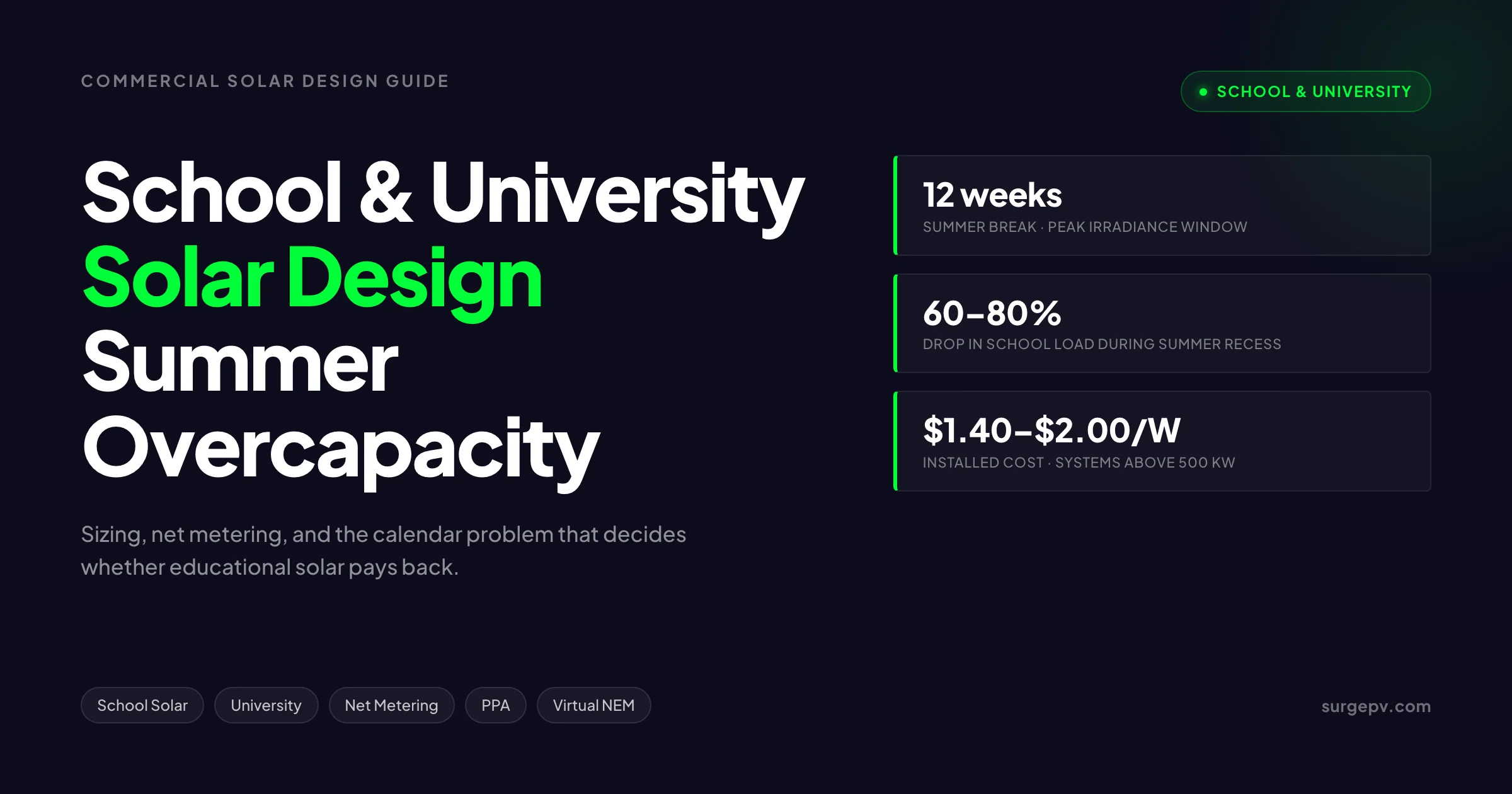
A typical K-12 school in the United States consumes around 8 kWh per square foot per year, about 60 percent of which is electricity (ENERGY STAR, 2024). Translate that to a 75,000 sq ft elementary school and you get roughly 360,000 kWh of annual electricity use. Easy to size a solar array for, except for one inconvenient fact — the building is closed for 10 to 12 weeks during the highest-irradiance months of the year. That is the summer overcapacity problem in school solar panel design, and it determines almost everything about how the system gets sized, how it gets financed, and whether it actually pays back.
Translate that to a 75,000 sq ft elementary school and you get roughly 360,000 kWh of annual electricity use. Most schools that get burned on solar economics are not victims of bad equipment. A K-12 school has a load curve that drops to roughly emergency-lighting and HVAC-minimum levels for two to three months while solar production is peaking.
TL;DR — School and University Solar Design
K-12 schools close for 8 to 12 weeks during peak solar months, so summer production overshoots building load by 60 to 80 percent. Net metering rules — annual true-up, monthly settlement, virtual aggregation — determine whether that surplus becomes value or waste. Size to academic-year consumption, model the summer export under local rules, and reach for storage or virtual net metering only when the rollover math fails.
Most schools that get burned on solar economics are not victims of bad equipment. They are victims of a design that ignored the calendar. This guide covers what solar design software has to do differently for educational facilities, the net metering structures that make or break the financial case, sizing math worked through a real K-12 example, the PPA-versus-ownership decision after the IRA direct-pay change, and where storage and carports actually move the needle. Everything is calibrated to the engineering reality of designing for a building that empties out for the third of the year when the sun is strongest.
In this guide:
- Why educational facilities have a unique load profile and what that means for sizing
- The summer overcapacity problem in numbers — production vs. consumption month by month
- Net metering structures and how each one treats summer surplus
- Sizing math worked through a 75,000 sq ft K-12 elementary school
- University design — bigger, more complex, less seasonal but still mismatched
- Roof, ground-mount, and carport tradeoffs for school campuses
- Battery storage and when it actually solves the summer problem
- PPA, lease, and ownership economics after IRA direct-pay
- Virtual net metering and meter aggregation for multi-building districts
- Eight common school solar design mistakes and how to avoid them
The School Load Profile Problem
The single largest mistake in school solar panel design is treating the building like any other commercial facility. It is not. A K-12 school has a load curve that drops to roughly emergency-lighting and HVAC-minimum levels for two to three months while solar production is peaking. That mismatch is structural, not solvable through panel selection or inverter tuning.
A typical academic-year load curve for a US elementary school looks like this:
| Month | School status | Approx. load (% of peak month) |
|---|---|---|
| January | In session, heating peak | 95% |
| February | In session | 90% |
| March | In session | 80% |
| April | In session | 75% |
| May | In session, cooling ramp | 90% |
| June | Closed (weeks 2-4) | 35% |
| July | Closed | 25% |
| August | Closed (weeks 1-3) | 30% |
| September | In session, cooling peak | 100% |
| October | In session | 85% |
| November | In session | 80% |
| December | Partial closure | 70% |
Source: composite from ENERGY STAR Portfolio Manager school benchmarks and Lawrence Berkeley National Laboratory school energy data (LBNL CBES, 2024).
Now overlay solar production. A south-facing rooftop array in Atlanta produces about 65 percent more in June than in December. In Phoenix, the spread is closer to 80 percent. The result: solar production peaks during the same months when the building is empty.
Pro Tip
Pull at least 18 months of interval data, not just monthly bills, before sizing a school solar system. Interval data shows whether the building actually runs HVAC during summer (some districts pre-cool for early teacher returns) or whether load truly collapses. The difference is often 15 to 25 percent of the design size.
Universities have a softened version of the same curve. Dorms empty out in May and June, then partially refill for summer session and conferences. Lab buildings and data centers run year-round at 70 to 90 percent of academic-year load. Athletic facilities ramp up. The result is a load curve that drops 25 to 35 percent in summer rather than 70 to 80 percent — still a mismatch, but a manageable one.
Use solar design software that can ingest 15-minute interval data and overlay production-vs-consumption curves before locking in array size. Skipping this step is how schools end up with 1.4 MW arrays that should have been 900 kW.
The Summer Overcapacity Problem in Numbers
To make the mismatch concrete, take a 500 kW DC system on a school in Sacramento with a 400,000 kWh annual load. The PVWatts model produces a typical monthly breakdown:
| Month | Production (kWh) | School load (kWh) | Surplus / (Deficit) |
|---|---|---|---|
| January | 38,500 | 38,000 | 500 |
| February | 47,000 | 36,000 | 11,000 |
| March | 70,200 | 32,000 | 38,200 |
| April | 81,500 | 30,000 | 51,500 |
| May | 87,000 | 36,000 | 51,000 |
| June | 88,500 | 14,000 | 74,500 |
| July | 92,000 | 10,000 | 82,000 |
| August | 84,000 | 12,000 | 72,000 |
| September | 70,000 | 40,000 | 30,000 |
| October | 55,500 | 34,000 | 21,500 |
| November | 38,000 | 32,000 | 6,000 |
| December | 32,000 | 28,000 | 4,000 |
| Annual | 784,200 | 342,000 | 442,200 |
Numbers above are illustrative only. Real production should be modeled with solar irradiance data from a TMY3 dataset for the actual site.
The system was sized to roughly cover annual consumption (a 1.15:1 production-to-load ratio is reasonable for sizing). But notice what happens between June and August: 228,500 kWh of surplus piles up while the school is closed, and total annual surplus reaches 442,200 kWh — well over the school’s actual annual usage. Whether that surplus translates to real bill savings depends entirely on the net metering structure. Also see: Us Residential Solar Market Trends 2026. For United States-specific compliance details, see United States arizona/phoenix. For United States-specific compliance details, see United States california/los-angeles.
This is why the design conversation has to start with the utility tariff, not the rooftop. A roof-first design produces a number. A tariff-first design produces an outcome.
Net Metering Structures and Their Impact on Schools
There are four flavors of net metering in active use across North America in 2026, and each one treats summer surplus differently. The choice of structure can swing a school’s payback period by three to five years.
1. Annual True-Up with Retail-Rate Rollover
Best case for schools. Excess kWh from one month carry forward at full retail value to offset deficit months. At the end of the 12-month true-up period, any remaining credit is either cashed out at avoided-cost rates (typically 4 to 8 cents/kWh) or forfeited.
Why it works for schools: the summer surplus rolls forward into September and October when school is back in session and load picks up. As long as the array is sized so annual production roughly equals annual load, the credit account stays close to zero and the school sees retail-rate value on every kWh.
States and utilities still offering this structure include parts of New York, Massachusetts, New Jersey, Illinois, and most of the Midwest. The full state-by-state map is tracked by DSIRE (2026).
2. Monthly Settlement at Retail
Worst case for schools. Each month is settled independently. Excess production gets cashed out at avoided-cost rates immediately rather than rolling forward. A school with 75,000 kWh of June surplus might receive $4,500 (at 6 cents/kWh) instead of the $11,250 of bill offset value (at 15 cents/kWh) that an annual structure would have delivered.
This is the structure New Hampshire moved to and the one California is essentially in under NEM 3.0 — though California’s calculation uses time-of-use export rates that are even lower in summer midday hours. Monthly settlement reduces the effective value of solar for a seasonally mismatched load by 30 to 45 percent relative to annual true-up.
3. Net Billing / Avoided-Cost Export (NEM 3.0 Style)
Energy consumed on-site is valued at the retail rate. Any energy exported to the grid is valued at a much lower rate set by the utility — usually based on hourly avoided cost, often less than 5 cents/kWh during summer midday.
For schools, this is functionally similar to monthly settlement but worse, because even within a school day there can be export periods. A closed school exports virtually 100 percent of midday production at low rates. The economics typically require pairing the solar with battery storage sized to shift midday production to evening discharge — adding 40 to 70 percent to project cost. For more on this topic, see Adding Battery Storage Services.
4. Virtual Net Metering / Meter Aggregation
A single solar array offsets consumption across multiple meters owned by the same entity. About 18 states allow some version of this for schools, with rules varying by distance limit (typically 2 to 5 miles), meter cap (often 10 to 20 meters), and tariff treatment (Paradise Solar Energy, 2026).
For school districts, this is the single most powerful tool. A district with 12 schools can install one 2 MW array on the high school’s flat roof and apply credits across all 12 buildings, sized to district-wide annual consumption. Critically, the load profile of 12 mixed-use buildings is much smoother than a single school — administrative offices and continuing-education centers run summer programs, and the aggregate load drops only 35 to 45 percent in summer rather than 70 percent.
See our virtual net metering glossary entry for the regulatory mechanics.
Design Rule
If virtual net metering is available in your state, design district-level rather than school-level. Aggregate load smooths the seasonal mismatch and increases optimal array size by 30 to 50 percent.
How to Size a School Solar System
The framework is straightforward but the inputs matter. Use this process for any K-12 or university project.
Step 1: Pull 18+ Months of Interval Data
Monthly bills hide everything important. Get 15-minute interval data from the utility. If the utility cannot provide it, install a temporary current transformer logger on the main service for at least 4 weeks during the school year and 2 weeks during summer recess.
Look at three things:
- Daily peak demand by month (drives demand charge analysis)
- Daytime baseline load during school days (drives self-consumption sizing)
- Daytime baseline load during summer recess (drives export risk)
Step 2: Model Production with TMY3 and Real Tilt
Use a TMY3 weather file for the closest NSRDB grid point. Don’t accept rough irradiance averages from rules of thumb. Run the layout through dedicated PV modeling software with the actual tilt, azimuth, shadow analysis, and DC:AC ratio. For schools with complex roofs, multi-string-MPPT inverters or DC optimizers usually win on energy yield.
A reasonable starting specific yield range for fixed rooftop systems in the continental US is:
- Southwest (AZ, NV, NM, southern CA): 1,750-1,950 kWh/kWp/year
- South (TX, FL, GA, AL, MS): 1,500-1,700 kWh/kWp/year
- Mid-Atlantic and Midwest: 1,250-1,450 kWh/kWp/year
- Northeast and Pacific Northwest: 1,100-1,300 kWh/kWp/year
Step 3: Size to Net Metering Reality
This is the step most designers skip. Run three scenarios:
| Scenario | Sizing target | Use when |
|---|---|---|
| Match annual load | Production = 100% of annual kWh | Annual true-up with retail rollover available |
| Match school-year load | Production = ~80% of annual (excludes summer) | Monthly settlement or net billing tariff |
| Match aggregate district load | District-wide kWh × allocation | Virtual net metering available |
For our 75,000 sq ft elementary school example with 360,000 kWh annual usage in a region with annual true-up:
- Sizing target: 360,000 kWh production
- Specific yield in the region: 1,400 kWh/kWp/year
- DC nameplate: 360,000 / 1,400 = 257 kWp
- Module count at 450W: 571 modules
- Required roof area: roughly 33,000 sq ft of usable roof at 5.7 W/sq ft
For the same school under a monthly net billing tariff, the right size is closer to 200 kWp — leaving room on the roof for a future 60 kW battery or carport addition rather than installing modules that will export at avoided-cost rates.
Step 4: Validate with the Generation and Financial Tool
Run the full financial model with the actual tariff structure. Most schools care about three numbers: net 25-year savings, simple payback, and Year 1 cash impact. The financial model should output all three under the actual tariff, not a generic retail rate.
Design a school solar system in one tool, not five
SurgePV combines layout, shading, energy modeling, and financial outputs in one cloud platform. Design a 500 kW K-12 system, run it under three different net metering tariffs, and compare payback in under an hour.
Book a DemoNo commitment required · 20 minutes · Live project walkthrough
For a direct comparison, see Arka 360 vs SurgePV.
University Solar Design — Bigger, Less Seasonal, Still Mismatched
Universities are a different design problem. The load is larger (research universities run 50,000 to 300,000 MWh per year), the building mix is varied (residence halls, lecture buildings, labs, athletic facilities, data centers), and the summer drop is smaller. But the design challenges are real.
Master-Plan Sizing
University projects are almost always portfolio plays. A typical state university with 4 million sq ft of building stock might have 20 to 40 candidate roofs and 5 to 10 candidate parking lots. The design question is not “how big is this one array” but “what is the optimal mix across the whole portfolio over 5 to 10 years of phased deployment.”
Phase 1 should target the buildings with:
- Newest roofs (15+ year remaining life)
- Highest year-round load (data centers, hospitals, research labs)
- Lowest shading complexity
- Closest to existing electrical infrastructure
A good rule of thumb: phase 1 should not exceed 25 percent of the eventual portfolio capacity. This lets the university validate the financial model before committing to the full deployment.
Lab Building Edge Cases
Research labs and HVAC-intensive buildings (animal facilities, BSL-3 spaces, clean rooms) run 24/7 at 60 to 90 percent of full load even in summer. These are excellent solar host sites because the on-site self-consumption fraction stays high regardless of net metering rules. A 1 MW array on a chemistry building with a year-round 800 kW baseload will consume essentially all production on-site.
Conversely, undergraduate residence halls have the worst load profile — peak load in winter (heating, indoor activity) and near-zero load in summer. Avoid putting solar on dorm rooftops unless the credits can be aggregated to other meters via virtual net metering.
Microgrid and Resilience Design
A growing number of universities are designing solar arrays as part of campus microgrids capable of islanding during grid outages. This adds requirements: protection coordination with the rest of the campus distribution, dispatchable storage, IEEE 1547-2018 compliant inverters with grid-forming capability, and typically a black-start-capable generator backup.
Microgrid-grade design adds 20 to 35 percent to project cost but provides resilience value that pure-grid-tied systems cannot. For research universities with critical infrastructure (greenhouses, biorepositories, server rooms), the resilience case is sometimes the primary economic driver.
Roof, Ground-Mount, and Carport Tradeoffs
School and university campuses typically offer three siting options. Each has design implications.
Rooftop Systems
Pros: cheapest per watt installed ($1.40 to $2.20/W for systems above 250 kW), no land use cost, shortest interconnection distances. Cons: limited by roof condition and remaining service life. A 10-year-old TPO roof with 10 years of life left is a non-starter for a 25-year solar project.
Design rules:
- Confirm structural capacity for 4 to 6 psf added load (ballasted) or 1 to 2 psf (penetrating)
- Match system life to roof remaining life — never install on a roof with under 10 years of remaining life
- Coordinate with the roofing contractor for warranty preservation
- Use aerial roof scan data for layout to catch obstructions, expansion joints, and slope variations
Ground-Mount Systems
Pros: optimal tilt and azimuth, easier maintenance access, larger system sizes possible, no roof conflicts. Cons: requires available land (rare on K-12 campuses, more available on university campuses), longer DC runs, sometimes triggers state SEPA review.
Most K-12 districts will not have ground-mount as an option. Universities frequently do — back lots, undeveloped portions of agricultural campuses, or athletic field perimeters.
Carport Systems
Pros: dual-use of existing parking, shade and weather protection for vehicles, EV charging integration opportunity, no roof warranty issues, optimal tilt achievable. Cons: $0.40 to $0.70/W premium over rooftop, structural cost dominates, requires steel design and foundation engineering.
For most universities and large K-12 campuses with surplus parking, carports are the smartest choice. A typical 200-space lot accommodates roughly 600 to 800 kW of solar at a per-watt cost of $2.10 to $2.80 — higher than rooftop but with several intangible benefits the school board will value: visible commitment, shaded parking as an amenity, and a natural pad for EV charging infrastructure that almost every district is planning anyway.
| Siting option | Cost ($/W) | System size range | Best for |
|---|---|---|---|
| Rooftop ballasted | $1.40-$2.00 | 100-1500 kW | Schools with newer flat roofs |
| Rooftop penetrating | $1.60-$2.20 | 50-1500 kW | Schools with sloped or older flat roofs |
| Ground-mount | $1.20-$1.80 | 250-5000 kW | Universities with available land |
| Carport | $2.10-$2.80 | 100-2000 kW | Campuses with surplus parking |
Battery Storage — When It Solves the Summer Problem
Storage is the most over-promised solution to school solar economics. The typical pitch is “store summer surplus and use it in winter.” That is not how lithium-ion batteries work. A 500 kWh battery cycled once a day delivers 182 MWh per year. A school with 250,000 kWh of summer surplus would need roughly a 700 kWh battery just to shift one day of summer overproduction into the next school day — and would need to do that for 60 consecutive days. The battery cost would exceed the value captured by 5 to 10 times.
What storage actually does well for schools:
1. Demand Charge Management
Most commercial school tariffs include a demand charge of $8 to $25/kW based on the highest 15-minute interval each month. A 200 kWh / 100 kW battery sized to discharge during the school’s afternoon peak (3-6 PM) typically pays for itself in 5 to 8 years through demand charge reduction alone — independent of net metering.
2. NEM 3.0 / Net Billing Optimization
In states with low export rates, storage absorbs midday production that would otherwise export at 4 to 6 cents/kWh and discharges it during the morning ramp (6-9 AM) or evening period when school maintenance and after-school programs run. This is the only economic case for storage on a school where summer load truly drops to near zero.
3. Resilience for Critical Loads
Schools designated as community emergency shelters often qualify for state and federal resilience funding to add storage. The economics rarely pencil on energy alone, but the incentives plus emergency-readiness mandate frequently close the gap.
4. Virtual Power Plant Participation
A growing number of utilities are paying schools $50 to $200 per kW per year to enroll batteries in dispatch programs. The school still uses the battery for its own load shifting most days but cedes dispatch control during grid stress events.
What storage does not do well: solve the seasonal mismatch. A battery sized to shift summer surplus to winter would cost more than the entire solar array. The right answer to seasonal mismatch is annual true-up net metering or virtual aggregation, not storage.
PPA, Lease, or Ownership — The Post-IRA Decision
For decades, the default school solar finance structure was a third-party PPA. Public schools are tax-exempt and could not directly use the federal Investment Tax Credit, so a developer would own the system and sell power to the school at a fixed kWh rate (typically 5 to 15 percent below the utility rate at signing).
The Inflation Reduction Act changed that calculus. The elective-pay (also called direct-pay) provision now lets tax-exempt entities — including public school districts — claim the ITC directly as a refundable cash payment from the IRS (2024). This shifted ownership economics dramatically.
| Structure | Upfront cost | Annual savings | 25-year NPV | Operational complexity |
|---|---|---|---|---|
| Direct ownership (with elective-pay ITC) | $0.95-$1.50/W after ITC | 100% of bill avoidance | Highest | School handles O&M |
| PPA (developer-owned) | $0 | 5-20% bill discount | Lower | Developer handles everything |
| Operating lease | $0-$100k/year | Mid-range | Mid | Shared O&M |
| C-PACE financing | $0 (assessment-financed) | 100% of bill avoidance | High | School handles O&M |
The general 2026 picture: schools with strong financial reserves and willingness to handle (or contract) O&M go with direct ownership and elective-pay. Schools with constrained budgets, limited bandwidth, or risk-averse boards still prefer PPAs. C-PACE works in states that authorize it for public schools (about 15 states currently).
For most large districts, the right answer is district-level ownership of one or two flagship systems plus PPA on the smaller, more complex sites. This gives the district direct ownership benefits where they matter most while avoiding the O&M overhead on every single roof.
Virtual Net Metering for Multi-Building Districts
Worth a deeper look because this is the single design lever that can make or break a district-level program. About 18 US states allow some version of virtual net metering for schools or municipal entities. The key design parameters vary widely:
| Parameter | Range across states |
|---|---|
| Maximum array size | 1 MW to 10 MW |
| Number of meters served | 4 to unlimited |
| Distance between array and offset meters | Same county to 2-mile radius |
| Allocation flexibility | Fixed at install vs. annually adjustable |
| Treatment of surplus | Retail credit, avoided-cost cashout, or forfeit |
| Eligible tariff classes | All meters vs. same class only |
For a school district, the highest-value approach is usually:
- Identify the building with the largest, newest, lowest-shading roof
- Confirm utility allows aggregation across all district meters
- Size array to district-wide annual consumption (typically 1.5 to 4 MW for a mid-size district)
- Allocate credits proportionally to each school’s prior-year usage
- Adjust allocations annually as building loads shift
A real example: a district with 10,000 students across 14 buildings would typically use 18 to 22 GWh/year. A 12-15 MW portfolio across 3 to 4 sites could cover 80 to 100 percent of district-wide consumption with annual aggregation. Phasing this over 5 years smooths capital outlay and lets the district learn from the first installs before scaling.
Common School Solar Design Mistakes
Eight mistakes that show up repeatedly in school solar projects, each one expensive enough to derail an otherwise good project.
1. Sizing to Annual kWh Without Checking Tariff
The single most common mistake. Designer sizes for 100 percent annual offset, assumes net metering will absorb seasonality, then discovers the local tariff is monthly settlement at avoided cost. Year-1 savings come in 30 to 40 percent below pro forma.
Fix: always model financials under the actual current tariff, with one sensitivity case for any pending tariff change.
2. Ignoring Roof Remaining Life
A 25-year solar project on a 12-year-old TPO roof with 13 years of remaining life is a project that will be removed and reinstalled at year 13 — adding $0.30 to $0.50/W in lifecycle cost the original financial model never captured.
Fix: independent roof condition assessment before any solar feasibility study. Replace the roof first (often grant-fundable separately) or move to ground-mount or carport.
3. Designing Around Architectural Preferences Instead of Production
School architects often want solar visible from the street for marketing, even when the production-optimal site is the back roof or the parking lot. Visible-but-suboptimal layouts can cost 15 to 25 percent of annual production.
Fix: separate the marketing question from the production question. Add a small visible array (10 to 20 kW) as an “education and demonstration” system, then put the bulk of the capacity in the production-optimal location.
4. Skipping Interval Data Analysis
Using monthly bills only, designers miss the actual demand profile — particularly summer break baseline, weekend load, and time-of-use opportunities. Fix: insist on 18 months of 15-minute interval data before final design.
5. Underestimating Interconnection Timeline
K-12 districts often plan installs around the summer break window. Utility interconnection studies for systems above 500 kW routinely take 9 to 18 months (DOE, 2024). A district that signs a contract in March hoping for a summer install is 6 to 12 months behind schedule before construction even bids.
Fix: file the interconnection application 12 to 18 months ahead of the desired commissioning date. Use the interconnection pre-application process where available to flag feeder capacity issues early.
6. Forgetting the After-Hours and Summer Programs Load
Some schools run summer enrichment programs, athletic camps, or community use that keep partial load during summer. Ignoring this load understates the value of summer production. Fix: get the facilities calendar from the district and model partial-occupancy summer load separately from full-closure weeks.
7. Inverter Selection That Forces a Single MPPT String
Schools with complex roof geometries (multiple azimuths, dormers, rooftop units) get killed by single-MPPT inverter designs. Module-level power electronics or multi-MPPT string inverters typically deliver 8 to 15 percent more annual yield. Fix: use shadow analysis software to identify how many distinct MPPT zones the site needs, then select inverters accordingly.
8. Treating Carports as Optional
Districts often default to rooftop because it’s “simpler” and never run the lifecycle numbers on carports. Carports add $0.40-$0.70/W in capital cost but eliminate roof-warranty conflicts, unlock larger system sizes, provide visible commitment, and create a foundation for EV charging. Fix: model carports as a default option in any school feasibility study, not a fallback.
Putting It Together — A District-Level Design Workflow
For a district considering a multi-school solar program, the right design sequence is:
-
Tariff analysis — Document the current net metering, demand charge, and time-of-use structure for every utility serving district buildings. Identify whether virtual net metering is available.
-
District-wide load study — Pull 18 months of interval data for all buildings. Build a district-wide aggregate load profile. Identify seasonal mismatch magnitude.
-
Site portfolio screen — Score every building roof and parking lot on roof age, structural capacity, shading, electrical proximity, and visibility. Rank.
-
Phase 1 sizing — Select the top 3 to 5 sites. Size each for the actual tariff structure and district-wide aggregation if available.
-
Financial model — Run direct ownership with elective-pay ITC, PPA, and lease scenarios for each site. Prefer ownership where O&M capacity exists.
-
Interconnection pre-application — File pre-applications 12+ months ahead of construction. Identify any feeder capacity issues that would constrain phase 2 sizing.
-
Procurement — Issue an RFP that specifies the design intent, leaves equipment selection to bidders, and requires bidders to model financials under the same tariff assumptions for apples-to-apples comparison. For France-specific information, see Agricultural Solar Case Study. For the latest details on France, see Floating Solar Farms France.
-
Phase 2 planning — Build phase 2 around what phase 1 actually produced rather than the original pro forma. Most districts find 10 to 20 percent of phase 1 assumptions need adjustment for phase 2.
This workflow takes 12 to 18 months from kickoff to phase 1 commissioning. Districts that try to compress it to 6 months almost always produce worse outcomes.
Real-World Case Examples
Three composite examples drawn from typical project patterns. Numbers are representative, not from a single specific project.
K-12 District, California (NEM 3.0 Tariff)
A unified school district with 8 elementary, 3 middle, and 2 high schools, total annual consumption 14 GWh. Initial solar proposal software output was 9 MW spread across 11 rooftops, sized to district-wide annual load under the assumption of legacy NEM 2.0 rates. NEM 3.0 took effect mid-design.
The redesign cut total array size to 5.6 MW (sized to school-day midday self-consumption) and added 4.5 MWh of battery storage across the four largest sites. The storage discharges during the 4-9 PM peak window when school buildings still draw load (after-school programs, athletics, custodial) and the export rate would have been near zero. Net result: project IRR landed at 9.2 percent versus the original 11.4 percent pro forma — lower than NEM 2.0 economics, but still above the district’s 7 percent hurdle. Without the storage redesign, IRR would have collapsed below 5 percent.
Mid-Size University, New York (Annual True-Up)
A 12,000-student state university with 2.4 million sq ft of building stock, 38 GWh annual consumption. Phase 1 deployed a 3.8 MW carport array over the main commuter parking lot, sized to roughly 35 percent of campus annual load. New York’s annual true-up at retail-rate rollover let the design ignore seasonal mismatch — surplus from June through August carried straight into September peak load.
The carport choice was driven by three factors: oldest residential building roofs were not solar-grade, the parking lot was the most visible site (sustainability was a stated brand value), and the structure created EV charging mounting points for a planned phase 2. Total project cost was $11.2 million ($2.95/W). With direct ownership and elective-pay ITC, the university received a $3.4 million IRS payment in year 2. Simple payback landed at 8.7 years.
Rural K-12 District, Iowa (Virtual Net Metering)
A consolidated rural district with 4 schools across 3 counties, total annual consumption 2.1 GWh. The district was the perfect virtual net metering candidate — Iowa’s investor-owned utilities allow aggregation across municipal-class meters within the same utility service territory.
Rather than four small school-by-school installs, the district built one 1.7 MW ground-mount array on 6 acres of unused land adjacent to the high school. Credits were aggregated across all 4 schools and the district administrative building. Per-watt cost dropped to $1.55 (single mobilization, no roof complications, single interconnection). Annual production covered 96 percent of district consumption. The project closed in 14 months from RFP to commissioning and the district avoided four separate roof assessments, four interconnection studies, and four sets of permits.
The lesson across all three: the design that wins is the one that respects the local tariff and the actual building portfolio, not the one that optimizes for a single rooftop.
Curriculum Integration and Brand Value
The economic case usually carries a school solar project, but the educational value often closes the political case. School boards approve projects faster when superintendents can describe how the array becomes a teaching asset.
Practical integration approaches:
- Live production dashboard in the main lobby, showing real-time kW, daily kWh, lifetime CO2 offset
- Data export API from the inverter monitoring system, feeding student-built data analysis projects in math and science classes
- Field trip access to the array (rooftop access requires safety planning; carport and ground-mount sites are easier)
- Career and technical education partnerships with local installers — students shadow O&M visits, learn IV-curve diagnostics
- Senior capstone projects modeling system performance, comparing to design predictions, identifying optimization opportunities
Universities go further. Engineering departments often use campus solar arrays as instrumented research platforms — bifacial vs. monofacial yield comparisons, soiling rate studies, inverter efficiency under partial shading. The data is real, the system is on-site, and the research informs the next phase of campus solar planning. For France-specific information, see France Solar Feed-in Tariffs. For more on this topic, see Bifacial Solar Panel Design Guide.
The brand value matters too. A high-visibility carport array on a main quad signals environmental commitment to prospective students and faculty in a way that an off-site PPA never can. For universities competing on sustainability rankings (AASHE STARS, Sierra Club Cool Schools, Princeton Review Green Honor Roll), on-campus generation is a measurable contributor.
Conclusion
School and university solar design is not commercial solar with a different roof. It is a different design problem driven by a calendar that empties the building during peak production months. Three things determine whether a school solar project actually saves money:
- Size to the tariff, not to annual kWh. Annual true-up with retail rollover lets you size to full annual load. Monthly settlement or net billing tariffs require sizing to school-year load only, leaving 20 to 30 percent of “available” roof unused.
- Use virtual net metering when available. A district-level array on the best site, with credits aggregated across all schools, almost always beats school-by-school designs on both economics and execution.
- Design with real interval data and real tariff structure. Generic specific yield numbers and assumed retail rates produce financial models that miss reality by 25 to 40 percent. Solar software that ingests interval data and models actual tariffs in the financial output is non-negotiable for serious school projects.
Get those three right and a typical school project pays back in 6 to 11 years and produces 20+ years of net positive cash flow. Get any of them wrong and the project either underperforms or becomes a cautionary tale that delays the district’s next project by a decade.
Frequently Asked Questions
Why do schools have a summer overcapacity problem with solar?
K-12 schools close for 8 to 12 weeks during peak summer irradiance. The solar array keeps producing at maximum output while the building load drops 60 to 80 percent. Without favorable net metering rollover or storage, those summer kilowatt-hours either get exported at low avoided-cost rates or get curtailed entirely. Universities have a smaller version of the same problem because dorms empty out and lab loads drop.
How do you size a solar system for a school?
Size the array to match annual academic-year consumption rather than peak load. A typical K-12 school uses 6 to 11 kWh per square foot per year. Pull 12 months of interval data, identify the load curve during the school year, and size the array so that academic-year production roughly equals consumption. Then check what happens to the summer surplus under your local net metering rules before finalizing the kWp number.
What is the best net metering structure for schools?
Annual true-up with retail-rate credit rollover is the best structure for schools because summer credits carry forward to cover winter consumption. Monthly true-up is the worst because excess summer credits get cashed out at avoided-cost rates that are typically 60 to 80 percent below retail. Virtual net metering and meter aggregation help districts spread one large array across multiple school buildings.
Should schools own their solar system or sign a PPA?
Most public schools cannot directly use the federal Investment Tax Credit because they are tax-exempt, so a third-party PPA or lease lets the developer monetize the credit and pass savings through. The IRA elective-pay (direct-pay) provision now lets tax-exempt entities claim the credit directly on owned systems, which has shifted many K-12 districts back toward ownership. Ownership wins on long-term economics; PPAs win on zero upfront cost and operational simplicity.
How much do solar panels cost for a school?
Commercial solar for schools runs $1.40 to $2.00 per watt installed for systems above 500 kW, and $2.00 to $3.50 per watt for smaller systems below 250 kW. A typical K-12 school installs a 250 to 750 kW system, so total cost lands between $400,000 and $1.5 million before incentives. After ITC and state incentives, the net is usually 30 to 50 percent lower.
How does battery storage solve the summer mismatch problem?
Storage helps two ways. Short-cycle batteries shift midday production into evening or early-morning use during the school year, capturing demand-charge savings that net metering does not address. Long-duration storage is rarely economic for purely seasonal shifts. The practical answer for most schools is a 1 to 2 hour battery sized for demand charge management, paired with whatever net metering rollover the utility offers.
Are carport-mounted solar systems worth it for schools?
Carports cost $0.40 to $0.70 per watt more than rooftop systems but they unlock parking-lot real estate that schools already have, provide shade for vehicles, and avoid roof-warranty conflicts. For universities and large K-12 campuses with surplus parking, carports often beat new rooftop installs on lifecycle economics, especially when paired with EV charging stubs.
What is virtual net metering and why does it matter for school districts?
Virtual net metering, also called meter aggregation, lets a single solar array offset consumption at multiple meters owned by the same entity. School districts use it to put one large array on the building with the best roof and apply credits across every school in the district. About 18 US states allow some form of virtual or aggregate net metering, with rules varying widely on distance limits and meter caps.