Quick Answer
The average US homeowner who installed solar in 2024 expected to save $1,400 per year on their electric bill. It is valued at the retail electricity rate because it displaces grid purchases. Under net billing, it may be worth $0.04–$0.12/kWh. Overestimating by 10–20% due to unmodeled shading Self-consumption ratio.
The average US homeowner who installed solar in 2024 expected to save $1,400 per year on their electric bill. Many saved less. Some saved more. The gap between expectation and reality is not random — it is determined by a small set of variables that most solar savings calculators handle poorly. Understanding those variables is the difference between an accurate estimate and a disappointed homeowner.
The average US homeowner who installed solar in 2024 expected to save $1,400 per year on their electric bill. It is valued at the retail electricity rate because it displaces grid purchases. Under net billing, it may be worth $0.04–$0.12/kWh.
This guide explains how electricity bill savings estimators work, what inputs matter, and how tariff structures — net metering, time-of-use rates, and feed-in tariffs — reshape the savings math in ways that generic calculators miss. Whether you are a homeowner evaluating solar, an installer building proposals, or a finance professional structuring project models, the framework here applies.
TL;DR — Electricity Bill Savings Estimator
A typical 6 kW residential solar system saves $900–$2,400 annually depending on local electricity rates and net metering policy. The savings come from two sources: self-consumed solar (valued at the full retail rate) and exported solar (valued at the net metering or net billing credit rate). In full net metering markets, savings equal approximately (annual production × retail rate) minus fixed charges. In net billing markets, savings depend heavily on self-consumption ratio and battery storage.
See Adding Battery Storage Services for detailed guidance.
In this guide:
- How electricity bill savings solar estimator tools work and what inputs drive accuracy
- System production and self-consumption: the two numbers that determine everything
- Net metering explained and its impact on savings by state
- Time-of-use (TOU) rates: why solar production timing no longer matches peak value
- Feed-in tariff vs. net metering: a global comparison
- Bill savings by tariff structure: flat rate, TOU, and dynamic pricing
- Bill savings by US state: net metering rules and real numbers
- Bill savings by country: Germany, Australia, UK, and Italy
- Seasonal variation in bill savings: summer surplus vs. winter deficit
- Escalation assumptions: why electricity rate growth changes the 20-year picture
- How batteries change the bill savings math
- When solar does not reduce your bill: the contrarian case Also see: solar panel ROI in Italy. Also see: Germany solar subsidies.
How Electricity Bill Savings Estimators Work
A solar bill savings estimator is a financial model that translates technical inputs into projected dollar savings. The core logic is simple. The implementation is not.
The Core Formula
Every savings estimator follows the same fundamental equation:
Annual Savings = (Self-Consumed kWh × Retail Rate) + (Exported kWh × Export Credit Rate) − Fixed ChargesBreaking this down:
Self-consumed kWh is solar production that flows directly to on-site loads. It is valued at the retail electricity rate because it displaces grid purchases. A kWh consumed on-site at $0.30/kWh saves $0.30.
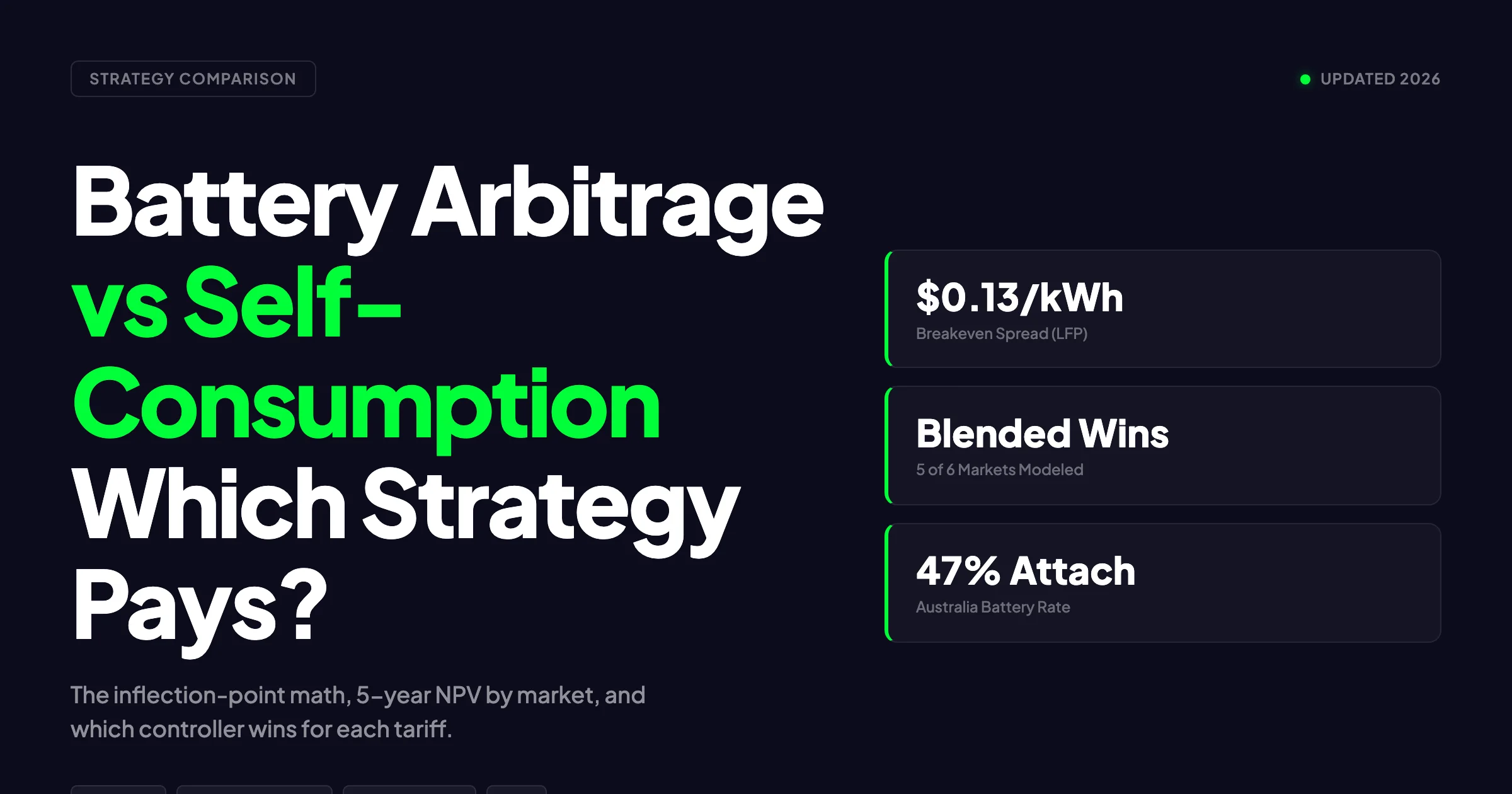
Exported kWh is surplus production sent to the grid. Its value depends on local policy. Under full net metering, it is worth the retail rate. Under net billing, it may be worth $0.04–$0.12/kWh.
Fixed charges are monthly connection fees, demand charges, and minimum bills that solar cannot eliminate. These range from $10–$50 per month depending on the utility.
Inputs That Drive Accuracy
| Input | Why It Matters | Common Error |
|---|---|---|
| Annual solar production | Determines total kWh available to save or export | Overestimating by 10–20% due to unmodeled shading |
| Self-consumption ratio | Sets the split between high-value self-consumption and lower-value exports | Assuming 70% when real households achieve 40–60% |
| Retail electricity rate | Values self-consumed kWh | Using state averages instead of actual tariff |
| Export credit rate | Values exported kWh | Applying outdated net metering rules |
| Fixed charges | Subtracts unavoidable costs | Ignoring monthly connection fees |
| Electricity rate escalation | Compounds savings over time | Assuming flat rates (understates 20-year savings by 25–35%) |
| System degradation | Reduces production 0.5–0.8% per year | Omitting degradation entirely |
| Inverter replacement | Major mid-life cost | Ignoring $1,500–$3,000 replacement at year 10–15 |
The Self-Consumption Problem
Self-consumption ratio is the most important and most miscalculated variable in solar savings estimation. It is the percentage of solar production consumed on-site rather than exported.
A typical US household without battery storage achieves 40–60% self-consumption. The remaining 40–60% exports to the grid. Why so low? Solar peaks at midday. Most households peak in the morning and evening.
| Household Profile | Typical Self-Consumption | Key Driver |
|---|---|---|
| Working couple, no kids, no battery | 35–45% | House empty during peak solar hours |
| Family with kids, someone home daytime | 50–65% | Midday laundry, cooking, AC load |
| Retirees, home all day | 55–70% | Continuous low-level consumption matches solar curve |
| Home office worker | 50–60% | Computer and HVAC load during solar hours |
| With 10 kWh battery | 70–85% | Battery stores midday surplus for evening use |
| With EV charging at home | 60–80% | EV charging during solar hours absorbs surplus |
Generic calculators often assume 70–80% self-consumption. This is realistic only for retirees with batteries or households with EVs charging during the day. For a typical working household, this assumption overstates savings by 20–30%.
Pro Tip
The fastest way to improve a savings estimate is to model self-consumption accurately. Use hourly load data if available. If not, apply a realistic self-consumption ratio based on household occupancy patterns. Never accept a calculator default without validating the assumption.
System Production and Self-Consumption Inputs
Before any savings calculation, you need two numbers: how much the system produces, and how much of that production the building consumes on-site.
Estimating Annual Solar Production
Annual production depends on system size, location, orientation, tilt, shading, and equipment efficiency. Read [Solar Shading Analysis Guide](/blog/solar-shading-analysis-guide) for a complete walkthrough.
The quick method: Multiply system size (kW) by the local production factor (kWh/kW/year).
| Region | Production Factor (kWh/kW/year) | 6 kW System Annual Yield |
|---|---|---|
| Southwest US (Arizona, Nevada) | 1,500–1,700 | 9,000–10,200 kWh |
| California | 1,400–1,600 | 8,400–9,600 kWh |
| Southeast US (Florida, Georgia) | 1,300–1,500 | 7,800–9,000 kWh |
| Northeast US (New York, Massachusetts) | 1,100–1,300 | 6,600–7,800 kWh |
| Pacific Northwest | 900–1,100 | 5,400–6,600 kWh |
| Germany | 900–1,100 | 5,400–6,600 kWh |
| Southern Italy | 1,400–1,600 | 8,400–9,600 kWh |
| Australia (Sydney, Perth) | 1,400–1,600 | 8,400–9,600 kWh |
| UK | 800–950 | 4,800–5,700 kWh |
Source: NREL PVWatts, PVGIS, and regional irradiance databases. Values for south-facing unshaded systems at optimal tilt.
The accurate method: Use simulation software like NREL PVWatts, PVGIS, or professional solar design software that models hourly production using satellite-derived irradiance data, temperature coefficients, and shading losses.
Production vs. Consumption: The Timing Mismatch
Solar production follows a bell curve peaking at solar noon. Household consumption follows a double-peak pattern: morning and evening. The overlap between these curves determines self-consumption.
A typical summer day for a 6 kW system in California:
| Time | Solar Production | Household Consumption | Net Flow |
|---|---|---|---|
| 6:00 AM | 0.3 kW | 0.8 kW | Import 0.5 kW |
| 9:00 AM | 3.5 kW | 1.2 kW | Export 2.3 kW |
| 12:00 PM | 5.2 kW | 1.5 kW | Export 3.7 kW |
| 3:00 PM | 4.8 kW | 2.0 kW | Export 2.8 kW |
| 6:00 PM | 2.1 kW | 3.5 kW | Import 1.4 kW |
| 9:00 PM | 0 kW | 2.8 kW | Import 2.8 kW |
On this day, the household self-consumed 4.5 kWh of solar and exported 8.8 kWh. Self-consumption ratio: 34%. This is typical for a working household without battery storage.
Improving Self-Consumption Without Batteries
Three strategies increase self-consumption before adding battery cost:
1. Load shifting. Run dishwasher, washing machine, and pool pumps during solar hours (10:00 AM–3:00 PM). Smart appliances with delay timers make this automatic.
2. Pre-cooling / pre-heating. In summer, cool the house to 72°F by 2:00 PM using solar, then let it drift to 76°F during evening peak rates. In winter, pre-heat thermal mass during solar hours.
3. EV charging at midday. A Level 2 EV charger draws 6.6 kW — enough to absorb most of a residential system’s midday surplus. Charging from 10:00 AM–2:00 PM instead of overnight can increase self-consumption by 15–25 percentage points.
Net Metering Explained and Its Impact on Savings
Net metering is the policy framework that determines how exported solar energy is valued. It is the single largest variable in solar savings estimation.
How Net Metering Works
Under net metering, the utility tracks energy flow in both directions through a bi-directional meter. At the end of the billing period:
- Energy imported from the grid is charged at the retail rate
- Energy exported to the grid is credited at the retail rate
- The customer pays only for the net difference
In a pure 1:1 net metering system, exporting 1,000 kWh and importing 1,000 kWh results in a zero energy charge. The grid acts as a free, infinite battery.
Net Metering vs. Net Billing
The distinction determines whether solar savings are generous or marginal.
| Feature | Full Net Metering (1:1) | Net Billing |
|---|---|---|
| Export credit rate | Full retail rate ($0.12–$0.45/kWh) | Wholesale or avoided-cost rate ($0.04–$0.12/kWh) |
| Grid as battery | Effectively free | Not available — exports are sold cheap |
| Battery value | Moderate | High — batteries avoid low-value exports |
| System sizing logic | Size to 100–120% of annual use | Size to 80–100% of annual use |
| Typical payback | 5–8 years | 8–14 years (without battery) |
| Annual savings (6 kW, $0.20/kWh) | $1,400–$1,800 | $900–$1,200 |
US Net Metering Status by State — 2026
| State | Net Metering Status | Export Credit | Key Detail |
|---|---|---|---|
| California | Net billing (NEM 3.0) | $0.05–$0.10/kWh (avg) | NEM 3.0 effective April 2023; export values vary hourly |
| New York | Full net metering | Full retail | Annual rollover; credits expire after 12 months |
| Massachusetts | Full net metering | Full retail | Cap raised to 10 kW for residential; SREC-II successor program active |
| New Jersey | Full net metering | Full retail | Strong SuSI successor to SREC market |
| Texas | Varies by utility | Retail to wholesale | No statewide policy; Oncor, CPS Energy offer net metering |
| Florida | Full net metering | Full retail | Net metering protected by voter-approved constitutional amendment |
| Arizona | Net billing (APS, SRP) | ~$0.10/kWh | APS moved to net billing in 2017; SRP followed |
| Hawaii | Net billing (all islands) | ~$0.10–$0.15/kWh | First state to end net metering (2015); battery adoption highest in US |
| Nevada | Restored net metering | Full retail | NEM restored in 2017 after public backlash against elimination |
| Illinois | Full net metering | Full retail | Through Ameren and ComEd; annual reconciliation |
| Alabama | No statewide NEM | None | Minimal solar policy; only TVA Green Power Providers |
| Tennessee | Minimal | Minimal | TVA programs limited; no statewide net metering |
Source: DSIRE database, state utility commission filings, and NREL State of the Market reports as of Q1 2026.
Key Takeaway — California NEM 3.0 Changed Everything
California’s NEM 3.0, effective April 2023, shifted the nation’s largest solar market from full net metering to net billing with hourly export values. Average export credits fell from ~$0.30/kWh to ~$0.08/kWh. This single policy change reduced simple payback periods from 5–6 years to 9–12 years for battery-less systems. It also made California the US leader in residential battery attachment rates — over 40% of new solar installations in 2025 included battery storage, up from 12% under NEM 2.0.
Time-of-Use Rates and Solar Production Timing
Time-of-use (TOU) rates charge different prices for electricity depending on when it is consumed. This creates a fundamental mismatch with solar production patterns.
How TOU Rates Work
Most US utilities with TOU structures use three periods:
| Period | Typical Hours | Rate Relative to Base |
|---|---|---|
| Off-peak | 10:00 PM–8:00 AM | 60–70% of base rate |
| Mid-peak | 8:00 AM–4:00 PM, weekends | 85–100% of base rate |
| On-peak | 4:00 PM–9:00 PM weekdays | 150–300% of base rate |
Solar panels produce most of their energy during mid-peak hours — when rates are moderate. They produce nothing during on-peak hours — when rates are highest.
The TOU Value Gap
In California PG&E territory (E-TOU-C tariff, 2026):
| Period | Rate | Solar Production | Value of Solar |
|---|---|---|---|
| Off-peak (12am–8am) | $0.16/kWh | None | N/A |
| Mid-peak (8am–4pm) | $0.24/kWh | High | Moderate |
| Peak (4pm–9pm) | $0.48/kWh | Declining to zero | Missed — no production |
A kWh of solar produced at 12:00 PM displaces $0.24/kWh mid-peak energy. But the household still imports $0.48/kWh peak energy at 7:00 PM. Without a battery, the solar does not address the most expensive energy.
Solar + Battery Under TOU
Adding a 10 kWh battery changes the math:
| Period | Rate | Solar Production | Battery Action | Net Result |
|---|---|---|---|---|
| Mid-peak (8am–4pm) | $0.24/kWh | High | Charge from solar | Store surplus |
| Peak (4pm–9pm) | $0.48/kWh | Declining | Discharge to home | Avoid peak imports |
| Off-peak (9pm–8am) | $0.16/kWh | None | Idle or trickle charge | Minimal activity |
The battery converts low-value midday solar into high-value peak displacement. Each kWh stored and discharged during peak hours saves $0.48 instead of earning $0.08 in export credits.
TOU Rate Impact on Annual Savings
| Scenario | Annual Savings (6 kW, California) | Payback Period |
|---|---|---|
| Solar only, flat rate | $1,500 | 7–8 years |
| Solar only, TOU without battery | $1,200 | 9–10 years |
| Solar + 10 kWh battery, TOU | $1,800 | 10–12 years (including battery cost) |
| Solar + battery + EV charging midday | $2,100 | 9–11 years |
Feed-in Tariff vs. Net Metering: A Global Comparison
Outside the US, solar savings mechanisms fall into two categories: net metering (or net billing) and feed-in tariffs (FiTs). The choice between them shapes national solar markets.
Feed-in Tariffs Explained
A feed-in tariff guarantees a fixed payment for every kWh of solar electricity produced — not just exported — for a contract term of 15–25 years. The rate is set by government policy, not the market.
| Country | FiT Status (2026) | Typical Rate | Contract Term |
|---|---|---|---|
| Germany | Active for small systems | €0.082–€0.090/kWh | 20 years |
| UK | Closed to new applicants | Legacy: £0.04–£0.14/kWh | 20–25 years |
| France | Active (prime à l’autoconsommation) | €0.10–€0.13/kWh | 20 years |
| Italy | Closed (Conto Energia legacy only) | Legacy: €0.12–€0.49/kWh | 20 years |
| Australia | State-based (minimal) | A$0.06–$0.20/kWh | Varies by state |
| Spain | Net billing for self-consumption | ~€0.06–€0.08/kWh export | N/A |
Net Metering vs. FiT: Which Delivers Higher Savings?
The answer depends on retail electricity rates and FiT levels.
Net metering wins when: Retail rates are high and rising. The US, Australia, and parts of Southern Europe fit this pattern. Self-consumption is valued at the retail rate, which typically exceeds FiT rates. Also see: European Solar Incentives. For Australia-specific compliance details, see Australia comparisons/lgc-vs-stc.
FiTs win when: Retail rates are low and FiT rates are set above market. Germany’s early EEG program (€0.50+/kWh in 2004) created a solar boom because the FiT far exceeded the retail rate. As FiTs have fallen to €0.08–€0.10/kWh, self-consumption plus net metering has become more attractive.
The German Case: From FiT to Self-Consumption
Germany illustrates the transition. In 2010, a homeowner received €0.33/kWh for every kWh produced under EEG feed-in tariff — far above the €0.24/kWh retail rate. The rational strategy was to export everything.
In 2026, the FiT is €0.082/kWh while retail rates are €0.35–€0.42/kWh. The rational strategy is now to self-consume as much as possible and export only surplus. German solar economics have inverted completely.
| Year | EEG FiT Rate | German Retail Rate | Optimal Strategy |
|---|---|---|---|
| 2010 | €0.33/kWh | €0.24/kWh | Export everything |
| 2015 | €0.13/kWh | €0.29/kWh | Mixed — self-consume + export |
| 2020 | €0.095/kWh | €0.32/kWh | Maximize self-consumption |
| 2026 | €0.082/kWh | €0.35–€0.42/kWh | Self-consume + battery |
Bill Savings by Tariff Structure
The same solar system produces dramatically different savings depending on the tariff structure it operates under. Here is a direct comparison. Read more about Agricultural Solar Case Study.
Assumptions for Comparison
- 6 kW residential system
- 9,000 kWh annual production
- 50% self-consumption (4,500 kWh)
- 50% export (4,500 kWh)
- Base retail rate: $0.20/kWh
Savings by Tariff Structure
| Tariff Type | Self-Consumption Value | Export Value | Fixed Charges | Annual Savings |
|---|---|---|---|---|
| Flat rate + full net metering | 4,500 × $0.20 = $900 | 4,500 × $0.20 = $900 | −$180 | $1,620 |
| Flat rate + net billing (50% retail) | 4,500 × $0.20 = $900 | 4,500 × $0.10 = $450 | −$180 | $1,170 |
| TOU + full net metering | 4,500 × $0.20 = $900 | 4,500 × $0.20 = $900 | −$180 | $1,620 |
| TOU + net billing | 4,500 × $0.20 = $900 | 4,500 × $0.08 = $360 | −$180 | $1,080 |
| Dynamic pricing + net billing | 4,500 × $0.22 = $990 | 4,500 × $0.06 = $270 | −$180 | $1,080 |
| No net metering (export blocked) | 4,500 × $0.20 = $900 | $0 | −$180 | $720 |
The gap between best-case (full net metering) and worst-case (no export) is $900 per year — more than 50% of total savings. This is why policy matters more than panel efficiency.
What Most People Get Wrong About Tariff Structures
Most homeowners assume their solar savings are determined by system size and sunlight. They are not. In most markets, the tariff structure explains 60–70% of the variation in savings between otherwise identical systems.
A 6 kW system in Massachusetts with full net metering and $0.28/kWh retail rates saves more than an identical system in Texas with net billing and $0.14/kWh rates — despite Texas having 20% more annual sunshine.
| Location | Annual Production | Retail Rate | Export Credit | Annual Savings |
|---|---|---|---|---|
| Massachusetts (6 kW) | 7,200 kWh | $0.28/kWh | Full retail | $1,850 |
| Texas (6 kW) | 8,600 kWh | $0.14/kWh | $0.06/kWh | $950 |
Massachusetts wins despite 16% less production because the value of each kWh is doubled.
Bill Savings by US State
Net metering rules vary by state, and so do savings. Here are realistic 2026 estimates for a 6 kW residential system.
State-by-State Savings Comparison
| State | Retail Rate ($/kWh) | Net Metering Policy | Export Credit | Annual Savings (6 kW) | Simple Payback |
|---|---|---|---|---|---|
| California | $0.28–$0.35 | Net billing (NEM 3.0) | $0.05–$0.10 | $1,100–$1,500 | 9–12 years |
| New York | $0.22–$0.26 | Full net metering | Full retail | $1,500–$1,800 | 6–8 years |
| Massachusetts | $0.26–$0.32 | Full net metering | Full retail | $1,700–$2,200 | 5–7 years |
| New Jersey | $0.18–$0.22 | Full net metering | Full retail | $1,300–$1,600 | 6–8 years |
| Texas | $0.12–$0.16 | Varies by utility | $0.04–$0.12 | $800–$1,200 | 8–12 years |
| Florida | $0.14–$0.18 | Full net metering | Full retail | $1,200–$1,500 | 7–9 years |
| Arizona | $0.13–$0.16 | Net billing | ~$0.10 | $900–$1,200 | 8–11 years |
| Hawaii | $0.38–$0.45 | Net billing | $0.10–$0.15 | $1,600–$2,200 | 6–8 years |
| Illinois | $0.14–$0.18 | Full net metering | Full retail | $1,200–$1,500 | 7–9 years |
| Colorado | $0.13–$0.16 | Full net metering | Full retail | $1,100–$1,400 | 7–9 years |
| Washington | $0.10–$0.12 | Full net metering | Full retail | $800–$1,000 | 9–11 years |
| Oregon | $0.12–$0.15 | Full net metering | Full retail | $950–$1,200 | 8–10 years |
| Nevada | $0.13–$0.16 | Full net metering | Full retail | $1,000–$1,300 | 7–9 years |
| North Carolina | $0.12–$0.15 | Full net metering | Full retail | $950–$1,200 | 8–10 years |
| Georgia | $0.12–$0.14 | Limited (Georgia Power) | ~$0.04 | $700–$900 | 10–13 years |
Assumptions: 6 kW system, 50% self-consumption, $3.00/watt installed cost, no battery. Savings include energy value only; incentive programs (ITC, state rebates, SRECs) reduce payback further. Source: EIA Electric Power Monthly, DSIRE, state utility commission data.
Why Hawaii Has High Savings Despite Net Billing
Hawaii is the exception that proves the rule. The state ended net metering in 2015 and moved to net billing. Yet solar savings remain among the highest in the US.
The reason is simple: electricity rates. At $0.38–$0.45/kWh, Hawaii’s retail rates are 2.5–3x the US average. Even with low export credits, every kWh of self-consumed solar displaces exceptionally expensive grid energy. A 50% self-consumption ratio in Hawaii saves more than an 80% self-consumption ratio in Texas.
This is the key insight for savings estimation: the product of (self-consumption × retail rate) usually matters more than total production.
Bill Savings by Country
Solar savings mechanisms differ fundamentally across national markets. Here is how four major solar markets compare.
Germany
Germany’s solar market runs on self-consumption plus EEG feed-in tariff for exports.
| Parameter | Value |
|---|---|
| Retail electricity rate | €0.35–€0.42/kWh |
| EEG feed-in tariff (2026) | €0.082–€0.090/kWh |
| Typical residential system | 8–10 kWp |
| Annual production (10 kWp) | 9,000–10,500 kWh |
| Self-consumption (no battery) | 30–45% |
| Self-consumption (with battery) | 60–75% |
Annual savings (10 kWp, no battery):
- Self-consumed: 4,000 kWh × €0.38 = €1,520
- Exported: 5,500 kWh × €0.085 = €468
- Total: €1,988/year
With 10 kWh battery:
- Self-consumed: 6,500 kWh × €0.38 = €2,470
- Exported: 3,000 kWh × €0.085 = €255
- Total: €2,725/year
The battery adds €737/year in savings — enough to justify the €4,000–€6,000 battery cost over 10–12 years.
Australia
Australia has high retail rates, excellent solar resource, and state-based feed-in tariffs.
| Parameter | Value |
|---|---|
| Retail electricity rate | A$0.28–$0.38/kWh |
| Feed-in tariff (varies by state) | A$0.05–$0.20/kWh |
| Typical residential system | 6.6–10 kW |
| Annual production (6.6 kW, Sydney) | 9,500–10,500 kWh |
Annual savings (6.6 kW, Sydney, no battery):
- Self-consumed: 4,500 kWh × A$0.32 = A$1,440
- Exported: 5,000 kWh × A$0.07 = A$350
- Total: A$1,790/year
Australian payback periods are among the shortest globally: 3–5 years for residential systems. The combination of high retail rates, strong sunshine, and falling installation costs (A$0.80–$1.20/Wp) makes Australian residential solar one of the world’s most mature markets. For Global-specific compliance details, see Global net-metering-by-country.
United Kingdom
The UK’s solar market operates without meaningful feed-in tariffs for new installations since the closure of the FIT scheme in 2019. For the latest details on UK, see Battery Solar System Design UK.
| Parameter | Value |
|---|---|
| Retail electricity rate | £0.30–£0.36/kWh |
| Export tariff (Smart Export Guarantee) | £0.03–£0.15/kWh |
| Typical residential system | 3–4 kWp |
| Annual production (4 kWp, south England) | 3,800–4,200 kWh |
Annual savings (4 kWp, no battery):
- Self-consumed: 1,800 kWh × £0.33 = £594
- Exported: 2,200 kWh × £0.07 = £154
- Total: £748/year
UK payback periods run 8–12 years. The small system sizes (limited by roof space and planning constraints) and moderate solar resource keep savings modest despite high retail rates.
Italy
Italy combines high retail rates, strong southern irradiance, and net metering via GSE. Read more about [Commercial Rooftop Solar Case Study Italy](/blog/commercial-solar-rooftop-case-study-italy-warehouse).
| Parameter | Value |
|---|---|
| Retail electricity rate | €0.27–€0.35/kWh |
| Scambio sul Posto (net metering) | €0.08–€0.13/kWh export credit |
| Typical residential system | 5–6 kWp |
| Annual production (6 kWp, Rome) | 8,000–8,800 kWh |
Annual savings (6 kWp, Rome, no battery):
- Self-consumed: 4,000 kWh × €0.29 = €1,160
- SSP credit: 3,500 kWh × €0.10 = €350
- Total: €1,510/year
Italian payback is 5–8 years with the 50% Detrazione Fiscale tax deduction. See our detailed solar panel ROI Italy analysis for regional breakdowns.
Global Savings Comparison Table
| Country | System Size | Annual Savings | Payback (No Incentives) | Key Mechanism |
|---|---|---|---|---|
| US (California NEM 3.0) | 6 kW | $1,100–$1,500 | 9–12 years | Net billing + TOU |
| US (Massachusetts) | 6 kW | $1,700–$2,200 | 5–7 years | Full net metering |
| Germany | 10 kWp | €1,990–€2,730 | 7–10 years | Self-consumption + EEG FiT |
| Australia | 6.6 kW | A$1,790 | 3–5 years | High retail + strong sun |
| UK | 4 kWp | £748 | 8–12 years | SEG export + self-consumption |
| Italy | 6 kWp | €1,510 | 5–8 years | SSP net metering + tax deduction |
Seasonal Variation in Bill Savings
Solar savings are not evenly distributed across the year. Summer overproduction and winter underproduction create seasonal cash flow patterns that matter for household budgeting.
Typical Monthly Production vs. Consumption
A 6 kW system in New York:
| Month | Solar Production | Household Use | Net Export/Import | Bill Impact |
|---|---|---|---|---|
| January | 420 kWh | 850 kWh | Import 430 kWh | −$108 |
| February | 510 kWh | 780 kWh | Import 270 kWh | −$68 |
| March | 680 kWh | 720 kWh | Import 40 kWh | −$10 |
| April | 820 kWh | 650 kWh | Export 170 kWh | +$43 |
| May | 900 kWh | 620 kWh | Export 280 kWh | +$70 |
| June | 950 kWh | 700 kWh | Export 250 kWh | +$63 |
| July | 930 kWh | 850 kWh | Export 80 kWh | +$20 |
| August | 880 kWh | 820 kWh | Export 60 kWh | +$15 |
| September | 780 kWh | 680 kWh | Export 100 kWh | +$25 |
| October | 650 kWh | 640 kWh | Export 10 kWh | +$3 |
| November | 480 kWh | 720 kWh | Import 240 kWh | −$60 |
| December | 400 kWh | 800 kWh | Import 400 kWh | −$100 |
| Annual | 8,400 kWh | 8,430 kWh | Net import 30 kWh | −$7 |
With full annual net metering, the summer export credits offset winter import costs. The homeowner pays approximately zero for energy over the year — plus fixed charges.
Seasonal Patterns by Climate
| Climate Type | Summer Production | Winter Production | Seasonal Swing | Key Consideration |
|---|---|---|---|---|
| Cold snowy (Minnesota, Maine) | High | Very low (60–70% below summer) | Extreme | Snow cover can reduce winter production 30–50% |
| Temperate (New York, Illinois) | High | Low (50–60% below summer) | High | Annual netting critical for economics |
| Mild winter (California, Oregon) | High | Moderate (30–40% below summer) | Moderate | More consistent year-round savings |
| Hot summer (Texas, Arizona) | Very high | Moderate | High | Summer AC load may absorb all production |
| Tropical (Florida, Hawaii) | Consistent | Consistent | Low | Minimal seasonal variation |
The Annual Netting Advantage
Utilities that offer annual net metering (rather than monthly) provide a significant economic benefit. Under monthly netting, summer export credits can only offset that month’s imports. Under annual netting, credits accumulate all year and offset winter imports.
| Netting Period | Summer Export Fate | Winter Import Fate | Annual Savings Impact |
|---|---|---|---|
| Monthly | Capped at monthly import | Full retail rate | −15–25% vs. annual |
| Annual | Roll over to winter | Offset by summer credits | Maximum savings |
| Real-time (no netting) | Sold at export rate | Bought at retail rate | −30–50% vs. annual |
Escalation Assumptions: Electricity Rates Rise Over Time
A savings estimate that assumes flat electricity rates is wrong. US residential rates have risen at an average of 2.8% per year since 2000. This compounding effect dramatically changes long-term savings.
Historical US Electricity Rate Growth
| Period | Average Annual Increase | Drivers |
|---|---|---|
| 2000–2010 | 2.2% | Fuel costs, infrastructure investment |
| 2010–2020 | 1.8% | Low natural gas prices, efficiency gains |
| 2020–2024 | 4.5% | Post-pandemic supply costs, grid modernization |
| 2024–2026 | 3.2% | Continued infrastructure investment |
| 20-year average (2000–2020) | 2.8% | Long-term baseline |
Source: EIA Electric Power Monthly, average US residential rates.
The Compounding Effect
At 3% annual escalation, a $0.20/kWh rate becomes:
| Year | Electricity Rate | Value of Self-Consumed Solar |
|---|---|---|
| 1 | $0.20/kWh | $0.20/kWh |
| 5 | $0.23/kWh | $0.23/kWh |
| 10 | $0.27/kWh | $0.27/kWh |
| 15 | $0.31/kWh | $0.31/kWh |
| 20 | $0.36/kWh | $0.36/kWh |
| 25 | $0.42/kWh | $0.42/kWh |
A kWh of solar self-consumed in year 20 saves $0.36 — 80% more than in year 1. Over 25 years, the average saved rate is $0.30/kWh, not $0.20/kWh.
Impact on 25-Year Cumulative Savings
| Scenario | Assumed Rate | 25-Year Cumulative Savings (6 kW) |
|---|---|---|
| Flat rate assumption | $0.20/kWh fixed | $28,000 |
| 2% annual escalation | Compounding | $35,000 |
| 3% annual escalation | Compounding | $40,000 |
| 4% annual escalation | Compounding | $46,000 |
Using a flat-rate assumption understates 25-year savings by 25–40%. Professional solar proposal software applies escalation curves of 2.5–3.5% to match historical trends.
Opinion: Most Calculators Understate Long-Term Savings
Most online solar calculators use flat-rate assumptions or minimal escalation (1–1.5%). This is conservative to the point of inaccuracy. Historical data supports 2.5–3% as a reasonable base-case assumption. The bias toward conservatism comes from a desire to avoid overstating savings — but systematic understatement is also misleading. A homeowner who expects $28,000 in savings and receives $40,000 is pleasantly surprised. But a homeowner who declines solar because the calculator showed marginal economics has missed a genuinely good investment.
How Batteries Change the Bill Savings Math
Battery storage is the most significant hardware variable in solar savings estimation. In net metering markets, batteries add modest value. In net billing and TOU markets, they are transformative.
Battery Economics: The Basic Math
A 10 kWh lithium iron phosphate (LFP) battery costs $6,000–$10,000 installed in 2026. What does it return?
In a full net metering market:
- Battery stores midday solar that would have exported at full retail credit
- Displaces evening grid imports at the same full retail rate
- Net value: minimal — the grid was already providing full credit
- Additional savings: $100–$300/year
- Payback: 20–30 years (not economically justified on savings alone)
In a California NEM 3.0 net billing market:
- Battery stores midday solar that would export at $0.08/kWh
- Displaces evening peak imports at $0.45/kWh
- Net value per kWh cycled: $0.37
- At 250 cycles/year (conservative): 2,500 kWh × $0.37 = $925/year
- Plus avoided fixed demand charges: $100–$200/year
- Additional savings: $1,000–$1,200/year
- Payback: 6–10 years
Battery Sizing for Maximum Savings
Oversized batteries waste money. Undersized batteries leave savings on the table.
| Household Profile | Recommended Battery | Daily Solar Surplus | Battery Utilization |
|---|---|---|---|
| Working couple, 6 kW solar | 5–7 kWh | 8–12 kWh | 40–60% |
| Family with kids, 8 kW solar | 10–13 kWh | 12–18 kWh | 55–75% |
| Retirees, 6 kW solar | 7–10 kWh | 6–10 kWh | 70–85% |
| Home office + EV, 10 kW solar | 13–16 kWh | 15–22 kWh | 60–80% |
Battery utilization matters. A 10 kWh battery that cycles 5 kWh per day (50% depth of discharge) delivers half the value of one that cycles 9 kWh per day. Proper sizing matches daily solar surplus to battery capacity.
The California NEM 3.0 Battery Boom
California’s NEM 3.0 created the clearest battery value proposition in US solar history. Battery attachment rates for new residential solar installations:
| Period | Battery Attachment Rate | Driver |
|---|---|---|
| NEM 2.0 (pre-April 2023) | 12–15% | Backup power, partial TOU arbitrage |
| NEM 3.0 transition (2023) | 35–40% | Immediate economic necessity |
| NEM 3.0 stable (2024–2025) | 42–48% | Established financial logic |
| 2026 (projected) | 50–55% | Battery cost decline + rate escalation |
California’s experience proves a policy point: when export credits fall far enough below retail rates, batteries become economically rational without subsidies.
Battery Degradation and Warranty Reality
LFP batteries degrade 1–2% per year. A 10 kWh battery with 6,000 cycle warranty at 80% retained capacity provides:
- Year 1 usable capacity: 10 kWh
- Year 10 usable capacity: 8.5 kWh
- Year 15 usable capacity: 7.5 kWh Also see: Us Residential Solar Market Trends 2026.
Savings estimates should account for this degradation. A battery that saves $1,000 in year 1 saves only $750 in year 15. Most professional models apply 1.5% annual capacity degradation to battery savings projections.
When Solar Does Not Reduce Your Bill
Solar is not universally beneficial. There are specific conditions where savings are minimal, delayed, or negated entirely.
Condition 1: Low Electricity Consumption
A household using 3,000 kWh/year at $0.12/kWh spends $360/year on electricity. Even a small 3 kW solar system producing 4,500 kWh/year cannot generate meaningful savings against a $360 baseline. The fixed costs of solar (inverter, installation, permitting) overwhelm the energy savings.
| Annual Use | Retail Rate | Annual Bill | Solar Savings Potential |
|---|---|---|---|
| 3,000 kWh | $0.12/kWh | $360 | Low — system cost exceeds savings |
| 3,000 kWh | $0.30/kWh | $900 | Moderate — high rate helps |
| 8,000 kWh | $0.12/kWh | $960 | Moderate — high consumption helps |
| 8,000 kWh | $0.30/kWh | $2,400 | High — ideal solar candidate |
Condition 2: Severe Shading
A system with 30% shading loss produces 30% less energy. If the savings estimate did not account for this, actual payback extends proportionally. A 7-year payback becomes 10 years.
Shading is the most common cause of solar underperformance. Trees, adjacent buildings, chimneys, and roof structures reduce production in ways that satellite imagery often misses. Professional shadow analysis before installation is essential.
Condition 3: Poor Net Metering or Net Billing
In markets with no export compensation, solar only saves what the household self-consumumes. A system producing 9,000 kWh/year with 50% self-consumption delivers only 4,500 kWh of savings. The other 4,500 kWh is wasted from a financial perspective.
Condition 4: Roof Replacement Required
If the roof needs replacement within 10 years, solar must be removed and reinstalled. This adds $2,000–$4,000 in costs that most savings estimates omit. A roof with 5 years of remaining life should be replaced before solar installation.
Condition 5: Frequent Moves
Solar payback assumes the homeowner stays in the property long enough to accumulate savings. A homeowner who moves in year 4 of a 7-year payback period has not broken even. Solar can increase property value — studies show $15,000–$20,000 for a owned system — but this is not guaranteed and varies by market.
The Narrative: When the Estimate Was Wrong
Mark and Lisa installed a 7 kW system in Phoenix in 2022. Their installer projected $1,800 in annual savings and a 6.5-year payback. Two years later, their actual savings averaged $1,100 per year.
What went wrong?
First, the installer used a 75% self-consumption assumption. Mark and Lisa both work in offices. Their real self-consumption was 42%. The midday solar surplus exported at SRP’s net billing rate of $0.10/kWh — not the $0.14/kWh retail rate assumed.
Second, the estimate assumed 1,650 kWh/kW/year production. Their west-facing roof with partial afternoon shading from a neighbor’s tree produced 1,420 kWh/kW/year — 14% below estimate.
Third, SRP increased fixed charges by $8/month in 2024. This $96/year increase was not in the original model.
The result: payback stretched from 6.5 years to 10.5 years. Not a bad investment — but not what was sold. Mark and Lisa’s experience is common. The gap between estimate and reality is usually 20–40%, driven by optimistic self-consumption assumptions and unmodeled shading.
Solar Bill Savings Estimator: Choosing the Right Tool
Not all savings calculators are equal. The right tool depends on your use case.
Calculator Types Compared
| Calculator Type | Accuracy | Best For | Key Limitation |
|---|---|---|---|
| Basic online (zip + bill) | ±30–50% | Initial curiosity | No shading, no actual tariff data |
| Satellite imagery (Google Project Sunroof style) | ±20–30% | Rough feasibility | Generic production factors; no tariff detail |
| Utility-specific calculator | ±15–25% | Preliminary planning | Often optimistic; may omit degradation |
| Professional solar design software | ±10–15% | Accurate proposals | Requires training; subscription cost |
| Custom financial model (Excel) | ±10–20% | Complex scenarios | Time-intensive; error-prone |
What to Look For in a Professional Estimator
A credible solar electricity savings calculator should include:
- Hourly production simulation — not just annual kWh estimates
- Actual utility rate structures — including TOU periods, tiers, and fixed charges
- Shading analysis — from satellite imagery or on-site measurement
- Realistic self-consumption modeling — based on household occupancy patterns
- Current net metering rules — not outdated policy assumptions
- Rate escalation — 2.5–3% annual increase as default
- System degradation — 0.5–0.8% per year
- Inverter replacement — mid-life cost at year 10–15
- Battery integration — if applicable, with realistic cycling assumptions
- Sensitivity analysis — best, base, and worst-case scenarios
Red Flags in Savings Estimates
| Red Flag | What It Means | Likely Impact |
|---|---|---|
| No shading analysis mentioned | Production may be overstated 10–30% | Payback 1–3 years longer |
| Self-consumption over 70% without battery | Unrealistic for working households | Savings overstated 20–30% |
| Flat electricity rate assumption | Ignores 25–35% of long-term value | 25-year savings understated |
| No inverter replacement cost | Omits $2,000–$3,000 mid-life expense | Payback 6–12 months longer |
| No degradation applied | Year 20 production = year 1 | Savings overstated 10–15% |
| Export credited at retail in NEM 3.0 market | Uses outdated policy | Savings overstated 40–60% |
Calculate Accurate Solar Savings with SurgePV
Model real utility rates, net metering rules, TOU structures, and battery economics for any US state or international market. Built for solar professionals who need defensible numbers.
Try the Financial ToolNo commitment required · Model any tariff structure · Export-ready proposals
Conclusion
Solar bill savings estimation is not guesswork. It is a structured financial model with known inputs and calculable outputs. The accuracy of the estimate depends entirely on whether the modeler respects the complexity of those inputs.
Three principles separate accurate estimates from misleading ones:
1. Self-consumption is king. The percentage of solar production used on-site matters more than total production. A smaller system with high self-consumption saves more than a larger system that exports most of its output at low credit rates.
2. Policy beats technology. Net metering rules explain more variation in solar savings than panel efficiency, inverter quality, or installation workmanship. A basic system under full net metering outperforms a premium system under net billing.
3. Time compounds everything. Electricity rate escalation, system degradation, and battery degradation all unfold over decades. A 25-year view with realistic assumptions produces a fundamentally different conclusion than a simple payback calculation.
For homeowners, the action is clear: use a calculator that models your actual utility rate structure, not a national average. For installers, the competitive advantage lies in proposal accuracy — the installer who sets realistic expectations builds referral business. The installer who overpromises builds review-site complaints.
For solar professionals building financial models, solar design software with integrated tariff databases, hourly production simulation, and battery economics is no longer optional. The gap between basic calculators and professional tools is the gap between disappointed customers and satisfied ones.
Frequently Asked Questions
How much will solar save on my electric bill?
Solar saves $800–$2,400 per year on a typical US residential electric bill. A 6 kW system in California at $0.32/kWh saves approximately $1,800–$2,200 annually. In Texas at $0.14/kWh, the same system saves $900–$1,100. The exact figure depends on your utility’s net metering policy, your household’s self-consumption rate, and whether you have time-of-use rates. Working households without batteries typically achieve 40–50% self-consumption. Households with batteries or EVs charging during the day reach 70–80%.
What is the difference between net metering and net billing?
Net metering credits exported solar at the full retail rate, so every kWh sent to the grid offsets one kWh of future consumption. Net billing credits exports at a lower rate — often the wholesale or avoided-cost rate. California’s NEM 3.0 is net billing where export values average $0.08/kWh versus $0.32/kWh retail. Net metering delivers higher savings. Net billing makes battery storage more valuable because storing and self-consuming avoids the low export credit.
How do time-of-use rates affect solar savings?
Time-of-use rates charge more during peak hours (typically 4pm–9pm) and less during off-peak hours. Solar produces most energy during midday off-peak hours when rates are lowest. This reduces export value unless you add battery storage to shift energy to peak evening hours. In California, peak rates reach $0.45–$0.52/kWh while solar exports credit at $0.05–$0.10/kWh. Batteries that discharge during peak hours convert low-value midday solar into high-value peak displacement.
Are solar savings calculators accurate?
Accuracy varies widely. Basic calculators using only zip code and bill amount can be off by 30–50%. Professional calculators using satellite imagery, hourly simulation, and actual tariff data achieve 10–15% accuracy. The most common error is overestimating self-consumption. Many calculators assume 70–80% when real households achieve 40–60%. Always verify the self-consumption assumption against your household’s actual occupancy pattern.
Do solar panels eliminate my electric bill completely?
Rarely. Most utilities charge a fixed monthly connection fee ($10–$25) that solar cannot offset. In net billing markets, exported energy is credited at below-retail rates, leaving a residual bill even with zero net annual consumption. A typical solar homeowner still pays $15–$60 per month in fixed charges and residual energy costs. Near-zero bills require solar plus battery storage and aggressive load-shifting in favorable rate structures.
How does battery storage change solar bill savings?
Batteries increase savings 20–40% in net billing and TOU markets by storing midday solar and discharging during peak evening rates. A 10 kWh battery in California NEM 3.0 can increase annual savings from $1,200 to $1,800. In full net metering markets, batteries add less value because the grid already provides full retail credit for exports. Battery payback ranges from 7–15 years depending on local rate structure.
Which US states have the best net metering for solar savings?
As of 2026, the best net metering states include New York, Massachusetts, New Jersey, and Illinois — all with full retail credit. California previously led but NEM 3.0 shifted to net billing with low export credits. States with the weakest solar economics include Alabama, Tennessee, and South Dakota, which lack statewide net metering policies.
How do electricity rate escalations affect long-term solar savings?
US residential rates have risen 2.8% per year on average over 20 years. At this rate, a $0.15/kWh rate becomes $0.25/kWh over 20 years. Solar savings compound because each self-consumed kWh avoids a progressively more expensive grid kWh. A calculator assuming flat rates understates 25-year savings by 25–35%. Professional models apply 2.5–3.5% annual escalation.