Quick Answer
A homeowner in Phoenix and a homeowner in Seattle both install identical 6 kWp solar systems. The Phoenix system produces 10,400 kWh per year. Import weather data — Typical Meteorological Year (TMY) files with hourly irradiance, temperature, wind speed, and humidity for the specific location 2.
A homeowner in Phoenix and a homeowner in Seattle both install identical 6 kWp solar systems. The Phoenix system produces 10,400 kWh per year. The Seattle system produces 6,600 kWh. Same panels. Same inverter. Same price. The only difference is location.
A homeowner in Phoenix and a homeowner in Seattle both install identical 6 kWp solar systems. The Phoenix system produces 10,400 kWh per year. Import weather data — Typical Meteorological Year (TMY) files with hourly irradiance, temperature, wind speed, and humidity for the specific location 2.
This 57% production gap is why every solar project starts with one question: how much will this system actually produce? Not the panel nameplate rating. Not the installer’s optimistic estimate. The real number, grounded in local solar resource, roof geometry, and physics.
A solar panel output calculator answers that question. It converts system capacity, location irradiance, orientation, and real-world losses into an annual kWh estimate. Installers use it for proposals. Homeowners use it to validate quotes. Financiers use it to underwrite loans.
This guide explains how output calculators work, what inputs matter most, where the errors creep in, and how to get an accurate estimate for any rooftop on earth.
TL;DR — Solar Panel Output Calculator
A solar panel output calculator estimates annual energy production by multiplying system capacity (kWp) by local solar irradiance, then applying a performance ratio (0.75–0.85) that accounts for temperature, shading, soiling, inverter losses, and wiring. A 6 kWp south-facing system in a sunny climate typically produces 8,500–11,000 kWh per year.
In this guide:
- How solar panel output calculators work — the math behind the estimate
- Solar irradiance by location — global data and what drives it
- Panel efficiency and degradation — how specs affect long-term output
- Temperature coefficient impact — why hot climates lose production
- Shading and orientation — the silent killers of solar yield
- Tilt angle and azimuth effects — finding the optimal geometry
- System losses — inverter, wiring, soiling, mismatch, and more
- Location-based output tables — US, Europe, and Asia examples
- How to use a professional output calculator in your workflow
- Common mistakes in output estimation — and how to avoid them
- What most guides miss about output calculators Also see: European Solar Incentives.
How Solar Panel Output Calculators Work
Every output calculator, from a simple spreadsheet to NREL’s PVWatts, follows the same fundamental equation:
Annual Energy (kWh) = System Capacity (kWp) × Specific Yield (kWh/kWp/year)
The specific yield is where all the complexity lives. It is not a single number. It is the product of location irradiance, system geometry, and a cascade of loss factors.
The Basic Formula
At its simplest:
Annual kWh = kWp × Irradiance (kWh/m²/year) × Performance Ratio
Where:
- kWp = system capacity under standard test conditions (STC)
- Irradiance = annual solar energy hitting a horizontal surface at the location
- Performance Ratio (PR) = the fraction of theoretical maximum that becomes actual output, typically 0.75–0.85
For a 6 kWp system in Los Angeles (1,850 kWh/m²/year) with PR = 0.82:
6 × 1,850 × 0.82 = 9,102 kWh/year
This is the back-of-envelope method. Professional calculators go deeper.
The Hour-by-Hour Simulation Method
Advanced calculators like PVWatts, PVsyst, and professional solar design software use hourly or sub-hourly simulation: For software options, see 7 Best PVsyst Alternatives in.
- Import weather data — Typical Meteorological Year (TMY) files with hourly irradiance, temperature, wind speed, and humidity for the specific location
- Calculate plane-of-array irradiance — for each hour, compute direct, diffuse, and reflected irradiance on the tilted panel surface using the Perez transposition model or similar
- Apply temperature model — cell temperature rises above ambient based on irradiance, wind speed, and mounting type (roof-mounted runs hotter than ground-mount)
- Apply module model — convert irradiance and cell temperature to DC power output using the module’s temperature coefficient, low-light performance, and spectral response
- Apply inverter model — convert DC to AC with inverter efficiency curve, clipping losses when DC exceeds inverter rating
- Apply system losses — wiring, soiling, mismatch, degradation, availability
- Sum hourly AC output — aggregate to annual, monthly, and daily totals
This method captures interactions that the simple formula misses. Temperature losses are higher in summer when irradiance is also higher. Shading losses vary by season and time of day. Inverter clipping only occurs during peak hours.
Standard Test Conditions vs. Real World
Panel wattage ratings are measured at STC:
- Irradiance: 1,000 W/m²
- Cell temperature: 25°C
- Air mass: 1.5
These conditions occur in the real world for only a few hours per year, if ever. A 400 W panel at STC might produce 320 W on a hot summer afternoon (cell temperature 65°C) or 420 W on a cold, clear winter morning with light snow reflection.
Output calculators bridge this gap by modeling how panel performance changes across the full range of real operating conditions.
Pro Tip
When comparing quotes from multiple installers, ask each for their estimated specific yield (kWh/kWp/year) and the performance ratio they assumed. A 10% difference in assumed PR changes annual production estimates by 10% — enough to shift payback calculations by months. Professional installers using solar design software will show you the hourly simulation breakdown, not just a single annual number.
Solar Irradiance by Location: The Primary Driver
Solar irradiance is the amount of solar energy striking a surface, measured in kWh per square meter per year (kWh/m²/year) or peak sun hours per day. It is the single most important input to any output calculator.
Global Solar Irradiance Map
| Region | Representative City | Annual GHI (kWh/m²) | Climate Type |
|---|---|---|---|
| Southwest US | Phoenix, AZ | 2,050–2,200 | Hot desert |
| Southern California | Los Angeles, CA | 1,800–1,950 | Warm Mediterranean |
| Southeast US | Miami, FL | 1,650–1,750 | Humid subtropical |
| Northeast US | Boston, MA | 1,400–1,550 | Humid continental |
| Pacific Northwest | Seattle, WA | 1,050–1,200 | Marine west coast |
| Northern Europe | London, UK | 950–1,100 | Temperate oceanic |
| Central Europe | Berlin, Germany | 1,050–1,150 | Temperate continental |
| Southern Europe | Madrid, Spain | 1,700–1,850 | Hot-summer Mediterranean |
| Middle East | Dubai, UAE | 2,000–2,150 | Hot desert |
| South Asia | Delhi, India | 1,750–1,950 | Semi-arid / monsoon |
| East Asia | Tokyo, Japan | 1,250–1,400 | Humid subtropical |
| Southeast Asia | Singapore | 1,550–1,650 | Tropical rainforest |
| Southern Africa | Cape Town, SA | 1,850–2,050 | Mediterranean |
| East Africa | Nairobi, Kenya | 1,900–2,100 | Highland / savanna |
| Australia | Sydney, Australia | 1,650–1,800 | Humid subtropical |
| Australia | Perth, Australia | 2,000–2,150 | Hot-summer Mediterranean |
Source: PVGIS (Photovoltaic Geographical Information System), European Commission JRC, and NREL Solar Resource Data. GHI = Global Horizontal Irradiance — total solar energy on a horizontal surface. For Global-specific compliance details, see Global net-metering-by-country. For Global-specific compliance details, see Global solar-permitting-speed-by-country.
What Drives Irradiance Differences
Latitude. Locations closer to the equator receive more direct sunlight year-round. At the equator, day length varies little and the sun passes nearly overhead at noon. At 60°N, winter days are short and the sun stays low in the sky, spreading the same energy over a larger surface area.
Cloud cover. Marine climates (Seattle, London) have persistent stratocumulus cloud layers that reflect 60–80% of incoming solar radiation back to space. Desert climates (Phoenix, Dubai) have clear skies 300+ days per year.
Altitude. Higher elevations receive more irradiance because the atmosphere is thinner. A site at 3,000 m elevation receives roughly 20–30% more clear-sky irradiance than a sea-level site at the same latitude. This is why the high Andes and Tibetan Plateau have exceptional solar resources despite their latitude.
Seasonal variation. Temperate locations show strong seasonal swings. Berlin in December receives roughly 0.5 kWh/m²/day. In June, it receives 5.5 kWh/m²/day — an 11× variation. Tropical locations like Singapore vary only 15–20% between wet and dry seasons. For Germany-specific information, see Community Solar Projects Germany. For more on this topic, see Community Solar Business Model.
From Horizontal to Tilted Surface
Output calculators do not use horizontal irradiance directly. They calculate plane-of-array (POA) irradiance — the energy hitting the tilted panel surface. POA irradiance depends on:
- Direct normal irradiance (DNI) — beam radiation from the sun’s disk
- Diffuse horizontal irradiance (DHI) — scattered radiation from the sky dome
- Ground-reflected irradiance — albedo (reflectivity) of the surface below the panels
- Tilt angle — angle of the panel from horizontal
- Azimuth angle — compass direction the panel faces (0° = north, 180° = south in northern hemisphere)
For a south-facing panel at optimal tilt, POA irradiance is typically 105–115% of horizontal GHI in mid-latitudes. The gain comes from better alignment with the sun’s path, especially in winter when the sun is low.
Key Takeaway
Irradiance data quality determines output calculator accuracy. Free tools using satellite-derived data (PVGIS, PVWatts) achieve ±5% for annual totals in most locations. Ground-station data improves this to ±3% for sites near weather stations. Always verify the weather dataset source when evaluating a calculator’s output — generic “national average” irradiance figures can be off by 20% or more for specific locations.
Panel Efficiency and Degradation: The Compounding Effect
Not all panels produce the same output from the same sunlight. Efficiency and degradation rate create long-term differences that output calculators must account for.
Module Efficiency Tiers (2026)
| Technology | Efficiency Range | Warranted Degradation | Typical Use Case |
|---|---|---|---|
| Standard monocrystalline PERC | 20–21% | 0.55%/year | Residential standard |
| TOPCon (Tunnel Oxide Passivated Contact) | 21.5–23% | 0.40%/year | Residential premium |
| HJT (Heterojunction) | 22–24% | 0.30%/year | High-end residential |
| IBC (Interdigitated Back Contact) | 23–24.5% | 0.35%/year | Premium / commercial |
| Bifacial (rear-side gain) | +5–20% additional | Same as monofacial | Ground-mount, elevated roofs |
Efficiency ranges represent commercially available modules in 2026. Laboratory cells exceed these values but are not yet mass-produced.
Higher efficiency matters in two ways. First, a 22% efficient panel produces more kWh per m² than a 20% efficient panel — 10% more from the same roof area. Second, higher-efficiency modules typically use newer cell architectures (TOPCon, HJT) with better temperature coefficients and lower degradation rates.
Degradation: The Hidden Cost
Solar panels lose output over time. A 0.5%/year degradation rate means a panel produces 88% of its original output after 25 years. A 0.3%/year rate means 93% after 25 years. That 5 percentage point difference, compounded over decades, is meaningful.
| Degradation Rate | Year 10 Output | Year 20 Output | Year 25 Output |
|---|---|---|---|
| 0.30%/year | 97.0% | 94.1% | 92.7% |
| 0.40%/year | 96.0% | 92.3% | 90.5% |
| 0.55%/year | 94.5% | 89.6% | 87.0% |
| 0.80%/year | 92.3% | 85.2% | 81.8% |
Most tier-1 manufacturers now warranty maximum 0.40–0.55%/year degradation. First-year degradation (light-induced degradation, LID) is typically 1–3% and occurs within the first weeks of operation. Output calculators apply this as a one-time loss in year 1, then the annual rate for subsequent years.
Bifacial Gain: Free Energy from the Back Side
Bifacial panels capture light reflected from the ground or roof surface behind the panel. The gain depends on: See Bifacial Solar Panel Design Guide for detailed guidance.
- Ground albedo — white gravel (0.60) > grass (0.20) > dark asphalt (0.10)
- Panel height — elevated panels capture more reflected light
- Row spacing — wider spacing reduces front-row shading of rear-side light on back rows
Typical bifacial gains:
| Installation Type | Bifacial Gain |
|---|---|
| Ground-mount, white gravel, 1.5 m height | 15–20% |
| Ground-mount, grass, 1.0 m height | 8–12% |
| Elevated flat roof (commercial) | 5–10% |
| Standard residential rooftop | 2–5% |
For output calculators, bifacial gain is added as a percentage uplift to the monofacial yield. Professional calculators model rear-side irradiance explicitly using view factor calculations.
Temperature Coefficient: Why Hot Climates Lose Production
Solar panels convert sunlight to electricity less efficiently as they heat up. This is one of the most misunderstood factors in output estimation.
How Temperature Affects Output
The temperature coefficient of power (Pmax) specifies how much output drops per degree Celsius above 25°C. For a typical monocrystalline panel:
Power loss = (Cell Temperature − 25°C) × Temperature Coefficient × System Capacity
Typical temperature coefficients:
| Module Technology | Temperature Coefficient (%/°C) |
|---|---|
| Standard PERC monocrystalline | −0.35 to −0.40 |
| TOPCon | −0.29 to −0.32 |
| HJT | −0.24 to −0.28 |
| IBC (Maxeon) | −0.29 |
On a 40°C ambient day in Phoenix, cell temperature on a roof-mounted system reaches 65–70°C. For a standard PERC panel (−0.38%/°C):
(70°C − 25°C) × 0.38% = 17.1% power loss
A 400 W panel produces 331 W at that temperature. The same panel on a 10°C day in Germany, with cell temperature of 30°C, loses only:
(30°C − 25°C) × 0.38% = 1.9% power loss
The Counterintuitive Finding
Hot climates have more irradiance but also more temperature loss. The net effect is that a panel in Phoenix produces more absolute kWh than the same panel in Berlin, but the gap is smaller than the irradiance difference alone would suggest.
| Location | Annual GHI | Avg. Cell Temp | Temperature Loss | Net Specific Yield |
|---|---|---|---|---|
| Phoenix, AZ | 2,150 | 48°C | 8.7% | 1,650 kWh/kWp |
| Los Angeles, CA | 1,900 | 38°C | 4.9% | 1,580 kWh/kWp |
| Berlin, Germany | 1,100 | 32°C | 2.7% | 980 kWh/kWp |
| Singapore | 1,600 | 45°C | 7.6% | 1,220 kWh/kWp |
Temperature loss calculated as annual average using hourly simulation with typical roof-mount conditions. Net specific yield = GHI × tilt gain × (1 − temperature loss) × PR, simplified.
Notice that Singapore has 45% more irradiance than Berlin but only 24% higher net specific yield. Temperature loss eats most of the irradiance advantage.
Mounting Matters
Roof-mounted systems run 15–25°C hotter than ground-mounted systems because the roof surface radiates heat upward. The air gap between panel and roof matters:
| Mounting Type | Typical Cell Temperature Rise Above Ambient |
|---|---|
| Ground-mount, open rack | +20–25°C |
| Elevated roof mount (>150 mm gap) | +25–30°C |
| Standard roof mount (50–100 mm gap) | +30–35°C |
| Building-integrated (BIPV, no gap) | +40–50°C |
For hot climates, choosing panels with lower temperature coefficients (TOPCon or HJT) and ensuring adequate ventilation gap can recover 3–5% of annual production.
Further Reading
For a deeper dive into how temperature affects panel performance, see our glossary entry on temperature coefficient. For irradiance terminology and measurement methods, see solar irradiance.
Shading and Orientation: The Silent Killers
Shading and suboptimal orientation are the two most common causes of underperforming systems. They are also the most frequently underestimated in output calculations.
Shading Loss Mechanics
Shading is not proportional. A panel with 10% of its surface shaded does not lose 10% of output. It can lose 30–50% because of how cells are wired in series.
In a standard string configuration, panels are wired in series. Current must flow through every panel in the string. If one panel is partially shaded, its current drops. The entire string’s current drops to match the shaded panel. One shaded panel can drag down 10–20 unshaded panels.
Modern mitigation techniques:
| Technique | How It Works | Typical Recovery |
|---|---|---|
| Bypass diodes | Allow current to skip shaded cell sections | 30–50% of shading loss recovered |
| Power optimizers | Module-level MPPT isolates shaded panels | 50–70% of shading loss recovered |
| Microinverters | Each panel has its own inverter | 60–80% of shading loss recovered |
| String inverter with 2+ MPPTs | Separate strings for shaded/unshaded areas | 20–40% of shading loss recovered |
Quantifying Shading Loss
Shading analysis requires 3D modeling of obstructions: trees, buildings, chimneys, HVAC equipment. The analysis produces a shading factor for each hour of the year.
Typical shading losses by obstruction type:
| Obstruction | Annual Loss (Typical) | Seasonal Pattern |
|---|---|---|
| Distant building (horizon) | 2–5% | Winter mornings/evenings |
| Nearby building (same height) | 10–20% | Winter dominant |
| Deciduous tree | 5–15% | Summer dominant (leaf-on) |
| Evergreen tree | 10–25% | Year-round |
| Chimney / vent pipe | 1–3% | Winter mornings/evenings |
| Self-shading (row-to-row) | 2–8% | Winter mornings/evenings |
A professional shading analysis using solar shadow analysis software models each obstruction’s shadow path across the roof throughout the year. The output is a shading loss percentage and, critically, a monthly shading profile — losses are typically 2–3× higher in winter when the sun is low.
Orientation and Azimuth Effects
In the northern hemisphere, south-facing panels produce the most annual energy. But “south” is not the only viable option.
| Azimuth (from South) | Output Loss vs. Optimal (at 35° tilt) |
|---|---|
| 0° (due South) | 0% (baseline) |
| ±15° (SSE/SSW) | 1–2% |
| ±30° (SE/SW) | 4–6% |
| ±45° (ESE/WSW) | 8–12% |
| ±60° (E/W) | 15–20% |
| ±90° (NE/NW) | 25–35% |
| 180° (North) | 40–50% |
East-west split arrays (common on gabled roofs) lose 10–15% of annual production compared to all-south, but they produce more evenly across the day. This can improve self-consumption for households with morning and evening demand peaks.
The installer story: A solar company in Colorado installed a 7.2 kWp system on a west-facing roof (azimuth 255°) because the south-facing roof was fully shaded by a neighbor’s tree. The west orientation cost 18% of annual production versus south-facing, but the absence of shading recovered 15% of that loss. Net result: 3% below optimal — a tradeoff the homeowner accepted to avoid tree removal costs of $3,500.
Tilt Angle and Azimuth: Finding the Optimal Geometry
Tilt and azimuth determine how well the panel surface aligns with the sun’s path. Output calculators apply correction factors or simulate hourly production based on these angles.
Optimal Tilt by Latitude
| Latitude | Optimal Year-Round Tilt | Winter-Optimized Tilt | Summer-Optimized Tilt |
|---|---|---|---|
| 20° (Mexico City, Hanoi) | 15–20° | 30–35° | 5–10° |
| 30° (Cairo, Shanghai) | 25–30° | 40–45° | 10–15° |
| 35° (Tokyo, Los Angeles) | 30–35° | 45–50° | 15–20° |
| 40° (Madrid, New York) | 35–40° | 50–55° | 20–25° |
| 45° (Bologna, Minneapolis) | 40–45° | 55–60° | 25–30° |
| 50° (London, Prague) | 45–50° | 60–65° | 30–35° |
| 55° (Edinburgh, Copenhagen) | 50–55° | 65–70° | 35–40° |
The rule of thumb — tilt equals latitude — is close for year-round optimization but slightly over-tilts for summer and under-tilts for winter.
Tilt Loss for Common Roof Pitches
Most residential roofs are not at optimal solar tilt. Common roof pitches and their tilt angles:
| Roof Pitch | Tilt Angle | Loss at 40°N Latitude (South-Facing) |
|---|---|---|
| Flat | 0–5° | 10–15% |
| Low-slope | 15° | 3–5% |
| Standard (4:12) | 18° | 2–4% |
| Medium (6:12) | 27° | 0–2% |
| Steep (8:12) | 34° | 0–2% |
| Very steep (12:12) | 45° | 3–5% |
At mid-latitudes (35–45°N), standard roof pitches (4:12 to 8:12) are within a few degrees of optimal. The loss is minimal. Flat roofs require tilted racking, which adds cost but recovers the production loss.
Seasonal Production Profiles by Tilt
A steeper tilt increases winter production at the expense of summer production. This matters for off-grid systems that must survive winter. For grid-tied systems, year-round optimization is usually best.
| Tilt | January (kWh/kWp) | July (kWh/kWp) | Annual (kWh/kWp) |
|---|---|---|---|
| 20° (summer-optimal) | 45 | 165 | 1,420 |
| 35° (year-round optimal) | 55 | 155 | 1,480 |
| 50° (winter-optimal) | 62 | 135 | 1,420 |
Example for 40°N latitude, south-facing, clear-sky model. Actual values vary by local climate.
System Losses: Where the Energy Goes
The performance ratio bundles all losses into one number. Understanding each loss category helps diagnose underperformance and improve design.
Loss Breakdown for a Typical Residential System
| Loss Category | Typical Range | Primary Driver |
|---|---|---|
| Temperature | 5–10% | Climate, mounting, module technology |
| Inverter efficiency | 2–5% | Inverter loading, part-load efficiency |
| Wiring (DC and AC) | 1–3% | Cable sizing, distance, temperature |
| Soiling | 2–8% | Climate, tilt angle, cleaning frequency |
| Shading | 0–15% | Obstructions, horizon, row spacing |
| Mismatch | 1–2% | Manufacturing tolerance, degradation variation |
| Availability | 0.5–2% | Inverter failures, grid outages, maintenance |
| Light-induced degradation (LID) | 1–3% (year 1 only) | Module technology |
| Spectral response | 0.5–2% | Module technology, atmospheric conditions |
| Angle-of-incidence | 2–4% | Fixed tilt vs. tracking |
| Total typical losses | 15–25% | PR = 0.75–0.85 |
Inverter Losses and Clipping
Inverters are not 100% efficient. A 98% efficient inverter loses 2% of all energy passing through it. But efficiency varies with load:
| Inverter Loading | Typical Efficiency |
|---|---|
| 10% load | 85–90% |
| 30% load | 94–96% |
| 50% load | 97–98% |
| 75% load | 98–99% |
| 100% load | 97–98% |
Inverter clipping occurs when DC panel output exceeds the inverter’s maximum AC output. This happens during peak sun hours on cold, clear days when panel output exceeds nameplate rating. A properly sized system clips 1–3% of annual production. Oversizing the DC-to-AC ratio (e.g., 1.2:1) is standard practice — the extra panels produce more energy in suboptimal conditions than they lose to clipping.
Soiling: The Neglected Loss
Dust, pollen, bird droppings, and pollution reduce light reaching the cells. Soiling loss varies dramatically:
| Environment | Annual Soiling Loss | Cleaning Frequency |
|---|---|---|
| Coastal, frequent rain | 1–2% | Rain-washed |
| Temperate, moderate pollution | 2–4% | Annual cleaning |
| Agricultural area, pollen/dust | 4–8% | 2–3× per year |
| Desert, sand/dust | 8–15% | Monthly cleaning |
| Industrial, heavy pollution | 10–25% | Weekly cleaning |
Tilt angle matters: panels steeper than 20° shed dust better than flat panels. Rain is an effective cleaner in most climates — a single heavy rain can recover 50–80% of soiling loss.
Mismatch and Degradation Variation
No two panels are identical. Manufacturing tolerance means a “400 W” panel might actually be 395–405 W. In a string, the lowest-current panel limits the entire string. Over time, panels degrade at slightly different rates, increasing mismatch.
Module-level power electronics (power optimizers, microinverters) eliminate string mismatch losses. For systems without MLPE, mismatch loss is typically 1–2%.
Location-Based Output Tables: Real Numbers
These tables show estimated annual production for a 6 kWp residential system under typical conditions.
United States: 6 kWp System Output by City
| City | State | Annual kWh | Specific Yield (kWh/kWp) | Key Factor |
|---|---|---|---|---|
| Phoenix | AZ | 10,200 | 1,700 | High irradiance, high temperature loss |
| Los Angeles | CA | 9,300 | 1,550 | Mild climate, moderate irradiance |
| San Francisco | CA | 8,400 | 1,400 | Marine layer reduces summer peak |
| Denver | CO | 9,000 | 1,500 | High altitude, clear skies |
| Miami | FL | 8,400 | 1,400 | High humidity, afternoon clouds |
| Atlanta | GA | 8,100 | 1,350 | Humid subtropical, moderate cloud |
| Chicago | IL | 7,200 | 1,200 | Cold winters, moderate summers |
| Boston | MA | 7,500 | 1,250 | Variable weather, decent summer |
| New York | NY | 7,800 | 1,300 | Moderate irradiance, urban heat |
| Seattle | WA | 6,600 | 1,100 | Persistent cloud cover |
| Honolulu | HI | 9,600 | 1,600 | Tropical, consistent irradiance |
Assumptions: South-facing, 30° tilt, standard PERC modules, 0.80 performance ratio, no significant shading. Source: NREL PVWatts v8, TMY3 weather data.
Europe: 6 kWp System Output by City
| City | Country | Annual kWh | Specific Yield (kWh/kWp) | Key Factor |
|---|---|---|---|---|
| Lisbon | Portugal | 10,200 | 1,700 | Highest irradiance in Western Europe |
| Madrid | Spain | 9,900 | 1,650 | Hot-summer Mediterranean |
| Rome | Italy | 9,300 | 1,550 | Strong southern irradiance |
| Athens | Greece | 10,500 | 1,750 | Excellent solar resource |
| Paris | France | 7,200 | 1,200 | Temperate, variable |
| Berlin | Germany | 6,600 | 1,100 | Northern latitude, moderate cloud |
| London | UK | 6,000 | 1,000 | Low irradiance, frequent cloud |
| Amsterdam | Netherlands | 6,300 | 1,050 | Maritime climate |
| Copenhagen | Denmark | 6,000 | 1,000 | High latitude, short winter days |
| Warsaw | Poland | 6,600 | 1,100 | Continental, cold winters |
Assumptions: South-facing, tilt = latitude, standard PERC modules, 0.80 performance ratio. Source: PVGIS SARAH-2 dataset, European Commission JRC.
Asia-Pacific: 6 kWp System Output by City
| City | Country | Annual kWh | Specific Yield (kWh/kWp) | Key Factor |
|---|---|---|---|---|
| Delhi | India | 9,600 | 1,600 | High irradiance, heavy pollution |
| Mumbai | India | 8,400 | 1,400 | Monsoon season reduces summer yield |
| Bangkok | Thailand | 9,000 | 1,500 | Tropical, consistent |
| Singapore | Singapore | 7,800 | 1,300 | Equatorial, afternoon thunderstorms |
| Tokyo | Japan | 7,200 | 1,200 | Humid, typhoon season |
| Sydney | Australia | 9,000 | 1,500 | Strong solar resource |
| Perth | Australia | 10,200 | 1,700 | Mediterranean climate, clear skies |
| Seoul | South Korea | 7,500 | 1,250 | Four seasons, moderate irradiance |
| Dubai | UAE | 10,800 | 1,800 | Desert, extreme irradiance |
| Nairobi | Kenya | 10,200 | 1,700 | Highland equatorial, minimal cloud |
Assumptions: South-facing (north-facing in southern hemisphere), tilt = latitude, standard PERC modules, 0.78 performance ratio (higher soiling assumed for some locations).
Monthly Production Profile Example
A 6 kWp system in Denver, Colorado (1,500 kWh/kWp/year specific yield):
| Month | kWh | % of Annual | Notes |
|---|---|---|---|
| January | 420 | 4.7% | Short days, low sun angle |
| February | 510 | 5.7% | Days lengthening |
| March | 720 | 8.0% | Spring equinox, snow reflection |
| April | 870 | 9.7% | Clear skies, moderate temps |
| May | 960 | 10.7% | Peak pre-summer |
| June | 1,020 | 11.3% | Longest days, some afternoon clouds |
| July | 990 | 11.0% | Monsoon moisture reduces peak |
| August | 930 | 10.3% | Still strong, shortening days |
| September | 810 | 9.0% | Excellent shoulder month |
| October | 690 | 7.7% | Fall clarity |
| November | 510 | 5.7% | Rapid decline |
| December | 420 | 4.7% | Shortest days, lowest sun |
| Annual | 9,000 | 100% |
The June:December ratio is 2.4:1. In Seattle, it is 4:1. In Singapore, it is 1.2:1. This seasonal variation is critical for off-grid battery sizing and for understanding why a system that “looks right” in summer might underperform in winter.
How to Use a Professional Output Calculator
Simple online calculators give a ballpark figure. Professional workflow demands more. Here is how experienced installers and designers use output calculators.
Step 1: Define the Site
Input the exact location — not the nearest major city. A suburb 20 km from the city center can have measurably different irradiance due to altitude, coastal influence, or urban heat island effects. Use GPS coordinates (latitude/longitude) for precision.
Step 2: Define the Array Geometry
Measure or model:
- Usable roof area — subtract setbacks, walkways, vents
- Tilt angle — measure with inclinometer or derive from roof pitch
- Azimuth — measure with compass app (correct for magnetic declination)
- Obstructions — photograph and measure tree heights, building distances, chimney locations Also see: Us Residential Solar Market Trends 2026.
Step 3: Select Equipment
- Module model — the exact panel matters for temperature coefficient, low-light performance, and degradation
- Inverter model — efficiency curve and clipping behavior vary
- Mounting system — affects ventilation and therefore temperature
Step 4: Run the Simulation
Professional solar design platform runs hourly simulations and outputs:
- Annual, monthly, and daily production
- Hourly generation profiles
- Loss breakdown by category
- Performance ratio
- Specific yield (kWh/kWp/year)
- 25-year production forecast with degradation
Step 5: Validate Against Reality
For existing systems, compare calculator output against actual production data from the monitoring system. Discrepancies reveal shading that was missed, soiling that is worse than assumed, or equipment underperformance.
The homeowner example: Sarah in Austin, Texas, used a free online calculator that estimated 9,600 kWh/year for her 6 kWp system. After year one, her monitoring showed 8,400 kWh — 12.5% below estimate. A professional shading analysis revealed that a neighbor’s tree had grown 2 meters since the Google satellite image was taken. The shading loss was 8%. Soiling on her flat 15° tilt roof added another 4%. The free calculator had assumed zero shading and 2% soiling. Real-world conditions matter.
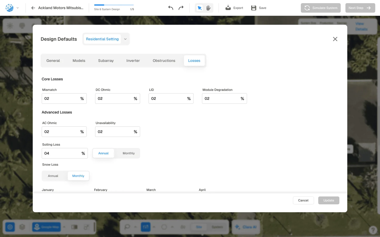
SurgePV’s losses panel breaks down every system loss category with location-specific defaults. Adjust each parameter based on site conditions for accurate output estimates.
Common Mistakes in Output Estimation
Even experienced designers make these errors. Avoiding them improves estimate accuracy by 10–20%.
Mistake 1: Using Nameplate Rating as Expected Output
A 6 kWp system does not produce 6 kW for 5 peak sun hours = 30 kWh per day. It produces 6 kW only at STC, which rarely occurs. The actual average output over daylight hours is 30–50% of nameplate rating. Annual production is nameplate × specific yield (1,000–1,800 kWh/kWp/year depending on location), not nameplate × hours of daylight.
Mistake 2: Ignoring Temperature in Hot Climates
Installers in Arizona, Texas, and the Middle East sometimes use PR = 0.85 because that is the textbook value. In 45°C ambient with roof-mount, PR is closer to 0.78. Using 0.85 overestimates production by 9%.
Mistake 3: Underestimating Soiling
“We get rain, so soiling is minimal.” Not always. Pollen season in the US Southeast creates a sticky film that rain does not fully remove. Agricultural dust in California’s Central Valley accumulates during dry months. Urban pollution in Delhi or Beijing creates a semi-permanent haze. Use location-specific soiling assumptions, not generic defaults. See our guide on 5kW Solar Panel Price in India for more.
Mistake 4: Assuming South-Facing When the Roof Faces East-West
A homeowner sees “south is best” and assumes their system will perform at 100%. Their roof faces southeast and southwest (common on gabled homes). The actual loss is 5–10% — not catastrophic, but enough to shift payback calculations.
Mistake 5: Using Annual Average for Off-Grid Sizing
Off-grid systems must survive the worst month, not the average month. A system sized for annual average production will fail in December. Off-grid calculators use the lowest-production month (typically December in northern hemisphere) as the design constraint.
Mistake 6: Forgetting Degradation in Long-Term Financial Models
A 25-year financial model that uses year-1 production for all 25 years overstates returns by 8–12%. Degradation compounds. Year 25 production is 85–93% of year 1, depending on module quality.
What Most Guides Miss About Output Calculators
Most articles on solar output calculators stop at the basic formula and a list of loss factors. Three important nuances are rarely discussed.
Nuance 1: The Performance Ratio Is Not a Constant
Textbooks quote PR = 0.80 as a rule of thumb. In practice, PR varies by:
- Climate: Hot deserts run 0.75–0.80. Temperate climates run 0.80–0.85. High-altitude clear-sky locations can reach 0.86–0.88.
- System age: PR degrades 0.3–0.5% per year due to module degradation, increased soiling, and inverter aging.
- Maintenance: A well-maintained system (annual cleaning, proactive inverter replacement) maintains PR 2–3% higher than a neglected system.
Using a single PR for all locations and all years is a $10,000 mistake on a commercial project.
Nuance 2: Hourly Profiles Matter More Than Annual Totals
Two systems with identical annual production can have radically different value. A west-facing system produces more in afternoon hours when electricity prices are highest under time-of-use tariffs. An east-facing system produces more in morning hours when grid demand is lower.
For self-consumption optimization, the hourly profile determines how much solar is used on-site versus exported. A system with a favorable hourly profile (peaking during household demand hours) can deliver 20% more economic value than a system with the same annual kWh but poor timing.
Professional cloud solar design tool outputs hourly generation profiles that feed directly into self-consumption and financial models. Annual kWh alone is insufficient for accurate ROI calculation.
Nuance 3: Satellite Irradiance Data Has Systematic Biases
Free calculators rely on satellite-derived irradiance (PVGIS, NSRDB, SolarAnywhere). These datasets are excellent for most locations but have known biases:
- Coastal fog: Satellites underestimate fog frequency, overestimating irradiance by 5–10% in coastal California, Peru, and Namibia.
- Mountain shadowing: 1 km satellite resolution misses valley shadowing, overestimating irradiance in steep terrain by 10–20%.
- Urban heat island: Satellite-derived temperature data may underestimate cell temperature in dense urban areas, under-predicting temperature losses.
For high-stakes projects (commercial, utility-scale), ground-station data or on-site measurement (pyranometer for 6–12 months) reduces uncertainty from ±8% to ±3%.
Opinion: The 80% Performance Ratio Myth
Industry training materials routinely quote 0.80 as the standard performance ratio. This number originated in central European conditions (Germany, Netherlands) in the 2010s. It is not universal. A rooftop system in Riyadh with roof-mount PERC modules, minimal cleaning, and 45°C summer ambient will struggle to achieve 0.75. A ground-mount system in the Atacama Desert with HJT modules and monthly cleaning can exceed 0.87. Treating PR as a constant is lazy engineering. Calculate it from first principles for every project.
Regional Comparison: Where Solar Output Varies Most
Understanding regional differences helps set realistic expectations and identify high-value markets.
Highest Output Regions (1,700+ kWh/kWp/year)
| Region | Why It Performs | Caveat |
|---|---|---|
| Southwest US (Arizona, Nevada) | Clear skies, high irradiance | Extreme temperature loss |
| Atacama Desert, Chile | Driest desert on Earth, minimal cloud | Remote, high altitude |
| Middle East (UAE, Saudi Arabia) | Desert climate, consistent | Dust soiling, extreme heat |
| Australia (Perth, Alice Springs) | Continental interior, clear skies | Bushfire smoke season |
| Southern Spain / Portugal | Mediterranean climate, low rainfall | Summer heat reduces efficiency |
| East Africa (Kenya, Ethiopia) | Equatorial, high altitude, minimal cloud | Infrastructure challenges |
Moderate Output Regions (1,200–1,600 kWh/kWp/year)
| Region | Characteristics |
|---|---|
| Southern Europe (Italy, Greece) | Strong solar resource, seasonal variation |
| Southeast US (Florida, Georgia) | Good irradiance, humidity and afternoon clouds |
| East Asia (Japan, Korea) | Moderate irradiance, four distinct seasons |
| Southern Africa (South Africa, Namibia) | Strong resource, winter-dominant rain |
| India (most regions) | High irradiance, monsoon reduces summer peak |
Lower Output Regions (800–1,200 kWh/kWp/year)
| Region | Challenge |
|---|---|
| Northern Europe (UK, Germany, Scandinavia) | High latitude, frequent cloud, short winter days |
| Pacific Northwest (Seattle, Vancouver) | Marine layer, persistent winter cloud |
| Northeast US (Boston, New York) | Variable weather, moderate irradiance |
| Southeast Asia monsoon regions | Heavy cloud during wet season |
| Equatorial rainforest (Amazon, Congo) | Persistent cloud cover despite latitude |
Model Solar Output for Any Location with SurgePV
SurgePV’s solar design software runs hourly production simulations using location-specific weather data, accurate shading analysis, and full loss modeling. Generate bankable output estimates for residential and commercial projects in any climate zone.
Book a DemoNo commitment required · 20 minutes · Live project walkthrough
The Tradeoff: Accuracy vs. Speed
Output calculators exist on a spectrum from quick estimates to engineering-grade simulations.
| Tool Type | Time Required | Accuracy | Best For |
|---|---|---|---|
| Rule-of-thumb (kWp × 1,500) | 30 seconds | ±25% | Initial feasibility |
| Online calculator (PVWatts, PVGIS) | 5–10 minutes | ±10–15% | Homeowner quotes, early-stage |
| Professional design software | 30–60 minutes | ±5–8% | Installer proposals, financing |
| PVsyst + custom meteorological data | 4–8 hours | ±3–5% | Utility-scale, due diligence |
| On-site pyranometer + modeling | 6–12 months | ±2–3% | Bankable projects, IPP tenders |
For residential installers, the sweet spot is professional SurgePV’s design suite that balances accuracy with speed. A 30-minute design session produces an estimate accurate enough for customer proposals and utility interconnection applications, without the days of work that PVsyst-level analysis requires.
For utility-scale projects, the cost of a 6–12 month on-site measurement campaign ($50,000–$200,000) is justified by the reduction in financing risk on a $50 million project.
Conclusion
Solar panel output calculators are not magic. They are physics models that convert sunlight data, panel specifications, and system geometry into energy production estimates. The quality of the output depends entirely on the quality of the inputs and the sophistication of the model.
Three principles for accurate output estimation:
- Use location-specific weather data, not rules of thumb. A 6 kWp system in Phoenix produces 57% more than the same system in Seattle. Generic “US average” numbers mislead both installers and customers.
- Model losses from first principles, not a single performance ratio. Temperature, soiling, shading, and inverter behavior interact in ways that a flat PR cannot capture. Hourly simulation with explicit loss categories produces estimates that match reality within 5–8%.
- Validate against actual production data. Every installed system is a calibration opportunity. Compare calculator predictions against monitored output. The gap reveals what the model missed — and makes the next estimate better.
For solar professionals, accurate output estimation is a core competency. It underlies every proposal, every financing application, and every customer expectation. Investing in professional AI solar design software with robust simulation engines, location-specific weather data, and detailed loss modeling pays for itself in fewer disputes, happier customers, and more competitive proposals.
For homeowners evaluating quotes, ask your installer for the specific yield estimate (kWh/kWp/year) and the performance ratio. If they cannot provide both, they are guessing. A professional using proper tools will show you the monthly production profile, the loss breakdown, and the weather dataset source. That transparency is the mark of a quality installation.
Tools & Further Reading
Continue exploring related SurgePV resources:
Frequently Asked Questions
How does a solar panel output calculator work?
A solar panel output calculator multiplies system capacity (kWp) by local solar irradiance (kWh/m²/year), then applies a performance ratio (typically 0.75–0.85) that accounts for temperature losses, inverter efficiency, wiring losses, soiling, shading, and mismatch. The result is estimated annual kWh production. For example, a 6 kWp system in Phoenix (2,100 kWh/m²/year) with an 0.82 performance ratio produces approximately 10,332 kWh/year.
What is the average solar panel output per day?
Average daily output depends on location and system size. A 1 kWp system produces roughly 2.5–5.5 kWh per day depending on latitude and climate: 2.5–3.5 kWh in northern Europe, 3.5–4.5 kWh in the central US, and 4.5–5.5 kWh in the desert Southwest or southern Spain. A typical 6 kWp residential system produces 15–33 kWh per day on average, with seasonal variation of ±40% between winter and summer.
How much do solar panels produce per month?
Monthly solar production varies by season. In a typical temperate climate, June production is 2.5–3× December production. For a 6 kWp system in Germany: January ~180 kWh, July ~720 kWh. For the same system in Arizona: January ~420 kWh, July ~1,020 kWh. Most calculators output monthly profiles using historical irradiance data rather than simply dividing annual production by 12.
What factors reduce solar panel output?
Key factors that reduce solar panel output include: temperature (output drops 0.3–0.5% per °C above 25°C), shading (even partial shade on one panel can disproportionately reduce string output), soiling (dust, pollen, bird droppings — 2–25% loss depending on climate), inverter efficiency (2–8% loss), wiring resistance (1–3% loss), module mismatch (1–3% loss), and degradation (0.4–0.8% per year). Orientation and tilt errors away from optimal can reduce output 5–20%.
How accurate are solar panel output calculators?
Professional solar output calculators using site-specific weather data achieve ±5–8% accuracy for annual production when inputs are correct. Accuracy depends on three things: the quality of the underlying weather dataset (satellite-derived vs. ground-station), the sophistication of the loss model (simple vs. hour-by-hour simulation), and the accuracy of user inputs (actual tilt, azimuth, and shading conditions). Free online calculators with generic inputs typically achieve ±15–20% accuracy. The most accurate results come from tools that use PVLib or similar simulation engines with TMY weather files.
What is a good performance ratio for solar?
A good performance ratio for residential rooftop solar is 0.78–0.85. Commercial systems with optimal design and maintenance can reach 0.83–0.88. Performance ratios below 0.75 indicate significant issues: shading, soiling, inverter undersizing, or wiring problems. Performance ratio above 0.90 is rare for real-world systems and may indicate measurement error or overly optimistic loss assumptions. The global average performance ratio for operational PV systems is approximately 0.80.
How does location affect solar panel output?
Location affects solar output primarily through solar irradiance, which varies by latitude, climate, and local weather patterns. A 1 kWp system in southern Spain (1,750 kWh/m²/year) produces roughly 75% more annually than the same system in Scotland (1,000 kWh/m²/year). Within a country, differences can be substantial: a 6 kWp system in Arizona produces ~10,500 kWh/year versus ~6,600 kWh/year in Seattle. Altitude also matters — high-altitude locations receive more clear-sky irradiance due to thinner atmosphere. Read more about Battery Solar System Design UK.
What is the difference between kWp and kWh in solar?
kWp (kilowatt-peak) is the maximum power output of a solar panel or system under standard test conditions (STC): 1,000 W/m² irradiance, 25°C cell temperature, and air mass 1.5 spectrum. It is a capacity rating, not a production measure. kWh (kilowatt-hour) is actual energy produced over time. A 6 kWp system does not produce 6 kWh per hour — it produces 6 kWh per hour only at peak conditions. Over a year, the same 6 kWp system might produce 8,000–11,000 kWh depending on location. The ratio of annual kWh to kWp is called the specific yield.
How do I calculate solar panel output for my roof?
To calculate solar panel output for your roof: (1) Determine your roof’s usable area and orientation using satellite imagery or on-site measurement; (2) Find your location’s annual solar irradiance from PVGIS, NREL PVWatts, or a local meteorological database; (3) Select panel wattage and calculate system capacity: number of panels × wattage ÷ 1,000 = kWp; (4) Apply the basic formula: Annual kWh = kWp × Irradiance (kWh/m²/year) × Performance Ratio (0.80 typical); (5) Adjust for your actual tilt and azimuth using a tilt/azimuth correction factor; (6) Subtract shading losses based on a shade analysis. For professional accuracy, use solar design software that runs hourly simulations with local weather data.
What is the best tilt angle for solar panels?
The best fixed tilt angle for solar panels is approximately equal to the location’s latitude, adjusted slightly lower (latitude minus 5–10°) for year-round optimization or higher (latitude plus 5–10°) for winter optimization. For example: at 40°N latitude (New York, Madrid), optimal year-round tilt is 30–35°. At 51°N (London, Berlin), optimal tilt is 40–45°. Flat roofs typically use 10–15° tilt to minimize wind uplift while maintaining reasonable production. Tracking systems eliminate the fixed-tilt compromise by following the sun’s path, increasing annual production 15–35% depending on latitude.