Quick Answer
Battery degradation in solar systems follows two paths: cycle aging (0.01–0.05% per cycle) and calendar aging (1–3% per year). LFP batteries degrade slower than NMC. Temperature is the primary accelerator — every 10°C above 25°C doubles degradation rate. Proper modeling uses 8,760-hour dispatch simulations with temperature correction.
Battery degradation modeling determines whether a solar storage system delivers its promised value in year 10 or falls short by 30%. A 15-year solar system paired with a battery bank that loses half its capacity before year 12 forces an unplanned replacement costing $8,000–$15,000. This guide explains how to predict capacity fade using physics-based models, compare real-world chemistry performance, and embed degradation assumptions into financial projections so your storage design matches reality.
Battery degradation in solar systems follows two paths: cycle aging (0.01–0.05% per cycle) and calendar aging (1–3% per year). LFP batteries degrade slower than NMC. Temperature is the primary accelerator — every 10°C above 25°C doubles degradation rate.
Battery degradation in solar systems follows two paths: cycle aging (0.01–0.05% per cycle) and calendar aging (1–3% per year). LFP batteries degrade slower than NMC. Temperature is the primary accelerator — every 10°C above 25°C doubles degradation rate. Proper modeling uses 8,760-hour dispatch simulations with temperature correction.
TL;DR
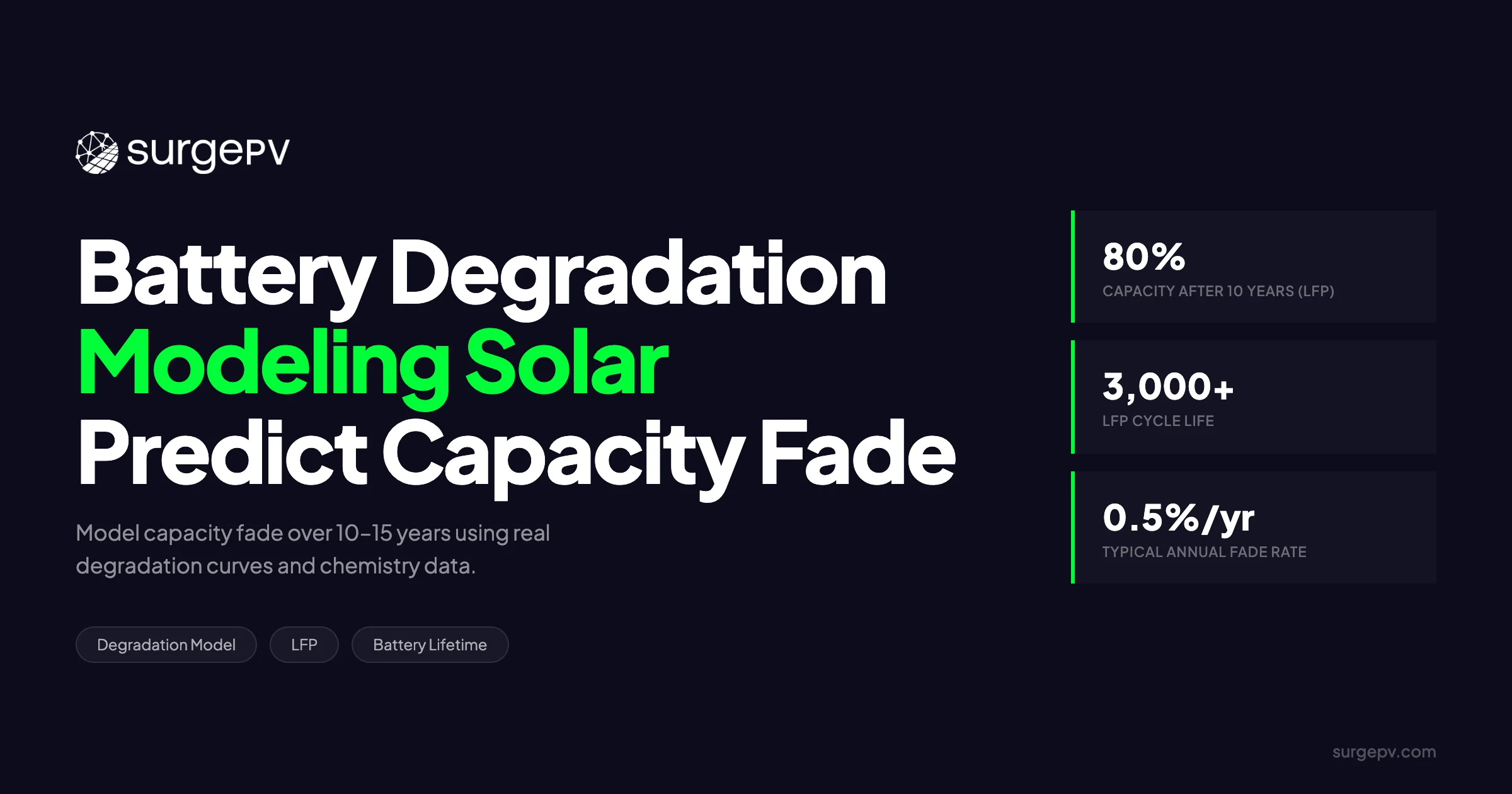
Battery degradation cuts usable capacity by 20–50% over 10–15 years. LFP fades slowest at 1–2%/year. The Arrhenius equation models temperature-driven fade. Tools like NREL BLAST predict capacity loss for lithium-ion chemistries under known thermal conditions. Solar designers who embed degradation into ROI models avoid under-sizing storage and warranty disputes.
In this guide, you will learn:
- How the Arrhenius equation predicts temperature-accelerated capacity fade
- Cycle-life comparison tables for LFP, NMC, NCA, and lead-acid
- Calendar aging vs cycle aging: which dominates in solar storage
- Four methods to measure State of Health (SoH)
- Real-world degradation data from Tesla Powerwall, LG ESS, BYD, Samsung SDI
- Why P50/P90 yield analysis fails without degradation modeling
- Financial thresholds for battery replacement timing
What Is Battery Degradation Modeling?
Battery degradation modeling is the process of quantifying how a battery loses usable capacity and gains internal resistance over time through physics-based equations and empirical data curves. It translates laboratory test results and field measurements into predictable capacity fade projections that solar designers can embed in lifetime performance simulations. Also see: Us Residential Solar Market Trends 2026.
Capacity fade in lithium-ion batteries stems from several interconnected chemical processes. Solid Electrolyte Interphase (SEI) layer growth on the anode consumes active lithium and increases resistance. Lithium plating deposits metallic lithium on the anode surface during fast charging or low-temperature operation. This permanently removes ions from circulation. Electrolyte oxidation at the cathode degrades the ionic transport medium. Active material loss occurs when cathode particles crack or detach from current collectors. This reduces the total sites available for lithium intercalation.
These mechanisms do not progress linearly. Degradation typically accelerates in early years as reactive surfaces are abundant, then slows as available material diminishes. Solar storage systems face two distinct aging pathways. Calendar aging proceeds during standby periods as chemical reactions occur regardless of use. Cycle aging accumulates with each charge and discharge event. Most grid-tied solar batteries spend 70–90% of their life in standby, which makes calendar aging the dominant factor engineers must model accurately.
solar proposal software must show clients realistic capacity projections instead of nameplate ratings. A 13.5 kWh battery marketed at 100% capacity will likely deliver 10.8 kWh by year 10 and 9.5 kWh by year 15 if degradation is modeled correctly. Modeling approaches fall into three categories. Semi-empirical methods like the Arrhenius equation combine temperature and time dependencies with fitted coefficients. Electrochemical models simulate ion transport and reaction kinetics at the particle level. Data-driven approaches use machine learning trained on fleet telemetry to predict fade for specific chemistries and operating profiles.
The Arrhenius Equation: How Temperature Drives Capacity Fade
The Arrhenius equation predicts how temperature accelerates battery degradation by describing the temperature dependence of chemical reaction rates. In lithium-ion cells, SEI layer growth follows a square-root-of-time (√t) dependence because the reaction rate slows as the layer thickens and acts as a diffusion barrier. The Arrhenius equation states k = A·e^(−Ea/RT), where k is the reaction rate constant, A is the pre-exponential factor, Ea is the activation energy, R is the gas constant, and T is absolute temperature in Kelvin.
For SEI growth in typical lithium-ion cells, Ea ranges from 50–70 kJ/mol (MDPI Batteries, 2026), with degradation fits to field data showing approximately 63 kJ/mol (UC Davis, 2021). This means a battery operating at 35°C degrades roughly twice as fast as the same battery at 25°C. In hot climates where outdoor enclosures reach 40°C internal cell temperature, the degradation rate can more than double compared to temperate conditions.
| Temperature | Relative Degradation Rate | Projected SoH at 15 Years (LFP) |
|---|---|---|
| 20°C | 0.7× | ~78% |
| 25°C | 1.0× (baseline) | ~72% |
| 30°C | 1.4× | ~65% |
| 35°C | 2.0× | ~58% |
| 40°C | 2.8× | ~50% |
The capacity fade curve follows a characteristic shape: steep in years 1–3 as fresh electrode surfaces react aggressively with electrolyte, then flat as reactive area diminishes and the SEI layer stabilizes. Solar designers must model this non-linear profile rather than assuming straight-line depreciation.
Outdoor battery enclosures in hot climates routinely exceed 35°C internal cell temperature even when ambient air stays below 30°C. Direct sun exposure on metal housings, poor ventilation, and heat generated during charge-discharge cycles all push cells past their optimal range. Designers who input rated specifications at 25°C into solar design software without correction produce optimistic capacity projections that fail in the field.
Cycle-Life Tables by Battery Chemistry
Cycle life varies by chemistry from under 1,500 cycles in standard NMC to over 6,000 in LFP. LFP’s stable olivine structure delivers the longest service life, while NMC trades longevity for higher energy density. Lead-acid falls shortest at 800–1,500 cycles. These differences determine whether a battery outlives the solar array or requires mid-life replacement.
Cycle life measures the number of equivalent full cycles a battery completes before reaching End of Life (EOL), conventionally defined as 80% of original capacity. Solar batteries rarely discharge 100% daily; instead they operate at partial cycles with Depth of Discharge (DoD) of 80–90%. Partial cycling extends calendar life because stress concentrates at specific SoC windows rather than the full electrode swing.
| Chemistry | Cycle Life (to 80% EOL) | Typical DoD in Solar | Calendar Fade/Year | Best Use Case |
|---|---|---|---|---|
| LFP (LiFePO₄) | 6,000–10,000 | 80–90% | 1–2% | Grid-tied residential, warm climates |
| NMC (LiNiMnCoO₂) | 1,500–3,000 | 80% | 2–3% | Space-constrained commercial |
| NCA (LiNiCoAlO₂) | 1,000–2,000 | 80% | 2.5–3.5% | High energy density, EV-derived |
| Lead-acid | 800–1,500 | 30–50% | 4–6% | Off-grid budget systems |
Lithium iron phosphate (LFP) degrades slowest because its olivine crystal structure remains mechanically stable during lithium insertion and removal. The strong phosphorus-oxygen bonds resist oxygen loss that plagues layered oxides. This structural integrity prevents the microcracking and cathode dissolution that accelerate fade in other chemistries. Manufacturer testing shows 6,000 cycles at 80% DoD to 60% EOL (BYD/Sunsynk, 2024), with some LFP systems rated for 8,000 cycles to 70% state of health (Eastmanworld, 2026).
Nickel manganese cobalt (NMC) offers higher energy density but suffers from microcracking in secondary particles as nickel-rich phases undergo anisotropic volume changes. Microcracks expose fresh surfaces to electrolyte, generating additional SEI growth and consuming active lithium. Manufacturer data typically rates NMC at 1,500–3,000 cycles to 80% EOL (Evenlite, 2024). This trade-off makes NMC suitable where rack space is limited but requires more conservative thermal management. For more on this topic, see Solar Racking Design Guide.
Lead-acid batteries fail primarily through sulfation, where lead sulfate crystals grow on plates during prolonged partial states of charge. In solar applications where batteries sit at high SoC for days, sulfation dominates and produces the shortest service life of any common chemistry.
Modern solar software should support chemistry-specific degradation curves because an NMC battery in Arizona degrades faster than an LFP battery in Germany even when both start at the same nameplate capacity. Also see: Germany solar subsidies.
Calendar Aging vs. Cycle Aging: Which Matters More in Solar Storage?
Calendar aging is the irreversible capacity loss that occurs while a battery sits idle, driven by continuous chemical reactions between electrode and electrolyte regardless of use. Cycle aging is the additional degradation caused by each charge and discharge event, including mechanical stress on particles, lithium plating during fast charging, and thermal excursions. In grid-tied solar, where batteries spend 70–90% of their life in standby at high state of charge, calendar aging typically dominates actual replacement timing.
A typical grid-tied solar storage profile involves 300–365 equivalent partial cycles per year and long standby periods at high State of Charge (SoC). At 300 cycles annually, an LFP battery rated for 6,000 cycles reaches its cycle-life EOL in 20 years. Calendar aging at 1.5% per year would reduce the same battery to 70% SoH in roughly 18–19 years. In this profile, calendar aging becomes the bottleneck that determines actual replacement timing.
Off-grid systems present a different picture. Deep daily cycling of 1.5 or more equivalent full cycles per year consumes 6,000 cycles in under 11 years. In this scenario, cycle aging dominates by year 8–10, especially if the battery operates at high C-rates or temperatures.
The practical implication for grid-tied designers is clear: prioritize thermal management and chemistry selection over cycle-count anxiety. A battery that can survive 10,000 cycles provides no value if calendar aging reduces it to 65% SoH in 12 years. Temperature control, shade for enclosures, and chemistry selection matter more than incremental cycle-life ratings for residential solar paired with storage. Shadow analysis software identifies shading issues before installation. Read Solar Shading Analysis Guide for a complete walkthrough.
How to Calculate State of Health (SoH)
State of Health (SoH) quantifies the remaining useful life of a battery relative to its new condition, expressed as present capacity divided by rated capacity. Accurate SoH tracking separates legitimate warranty claims based on actual degradation from disputes rooted in measurement error or optimistic manufacturer assumptions.
Four methods measure SoH with varying precision and equipment requirements:
1. Capacity Ratio
SoH = (Q_measured / Q_rated) × 100%
A full charge-discharge test under controlled conditions measures present capacity against the nameplate rating. This is the reference standard but requires taking the battery offline for several hours.
2. Internal Resistance Growth
SoH_R = (R_EOL − R_present) / (R_EOL − R_new) × 100%
Rising internal resistance reduces power capability and increases heat generation. DC pulse tests or electrochemical impedance spectroscopy track this parameter.
3. Coulombic Efficiency (CE)
CE = Q_discharge / Q_charge
In healthy lithium-ion cells, CE stays above 99.5%. Sustained readings below this threshold signal lithium plating or electrolyte decomposition.
4. Incremental Capacity Analysis (ICA) / Differential Voltage Analysis (DVA)
Plotting dQ/dV against voltage reveals peaks corresponding to specific phase transitions in electrode materials. Peak shifting or height reduction indicates active material loss and can predict failure before capacity drops significantly.
| Method | Equipment | Accuracy | Best For |
|---|---|---|---|
| Capacity Ratio | Battery cycler | ±1% | Warranty testing, lab validation |
| Internal Resistance | DC pulse tester, EIS | ±3% | Power capability assessment |
| Coulombic Efficiency | Precision coulomb counter | ±0.1% | Early fault detection |
| ICA/DVA | Cycler with dQ/dV logging | ±2% | Diagnostic analysis, research |
Battery Management Systems (BMS) report SoH using embedded algorithms, but these estimates can drift ±5% without periodic calibration against full capacity tests. Solar maintenance contracts should include annual SoH verification to keep projections accurate.
Real-World Degradation Data: Powerwall, LG ESS, BYD, Samsung SDI
Field data from independent test centers and warranty filings validates laboratory projections and exposes the gap between ideal test conditions and actual installation environments. The following data comes from accelerated cycling trials, academic fleet studies, and manufacturer technical disclosures that reflect real-world thermal and electrical stress.
Tesla Powerwall 3 (LFP, 2024–present)
Tesla’s Powerwall 3 switched to LFP cells, while the earlier Powerwall 2 used NMC chemistry. The Powerwall family carries a 10-year warranty guaranteeing 70% capacity retention at the battery AC output (Tesla, 2025). Independent telemetry analysis shows roughly 1.5–2% annual capacity fade in moderate climates for LFP-based units (Solar Insure, 2026). This projects to 70–75% SoH at year 10, comfortably within the warranty threshold. Hot-climate units in Arizona and Texas show 2.2–2.5% fade, pushing closer to the warranty boundary.
LG RESU (NMC)
LG Chem’s RESU series uses NMC chemistry. Warranty terms for the RESU 10H specify 60% retained capacity at 10 years or 22.4 MWh throughput, whichever comes first (EnergySage, 2024). Field data from European installations at 25°C average projects approximately 62% SoH at 10 years. Australian installations at 28–30°C average trend toward 55–58%. Also see: European Solar Incentives. For Australia-specific compliance details, see Australia comparisons/lgc-vs-stc.
BYD B-Box (LFP)
BYD’s LFP systems in Australian field conditions routinely experience 30°C+ average enclosure temperatures. Independent testing by ITP Renewables projects approximately 75% SoH after 10 years of daily cycling (SolarQuotes/ITP, 2019). BYD warranties 60% at 10 years, leaving moderate headroom. Read more about Solar Energy in Australia.
Samsung SDI (NMC)
ITP Renewables independent testing of the Samsung AIO10.8 showed 87% capacity retention after 1,808 equivalent full cycles under controlled conditions (ITP Renewables, 2020). Extrapolated to solar profiles with partial cycling and calendar aging in moderate climates, this suggests approximately 65% SoH at 10 years.
| Product | Chemistry | Observed Fade/Year | Projected SoH @ 10 Yrs | Climate Condition |
|---|---|---|---|---|
| Tesla Powerwall 3 | LFP | 1.5–2% | 70–75% | Moderate (15–25°C) |
| LG RESU | NMC | 2.5–3% | ~62% | Temperate (25°C) |
| BYD B-Box | LFP | ~2.5% | ~75% | Warm (30°C+) |
| Samsung SDI | NMC | 2–2.5% | ~65% | Moderate (25°C) |
The gap between lab-cycle projections and field reality is substantial. Laboratory tests often ignore calendar aging by running continuous cycles over months rather than years. In real solar installations, calendar aging dominates and produces faster fade than cycle-count extrapolation predicts.
P50/P90 Yield Impact: How Degradation Affects Solar System Output
P50 and P90 are probabilistic metrics borrowed from solar irradiance analysis and applied to storage capacity, where P50 represents the median expected capacity and P90 is the conservative estimate exceeded with 90% probability. Ignoring degradation in these metrics causes financial models to overestimate available storage by 15–25% in year 10, cascading into erroneous ROI projections and payback periods.
When designers model batteries at 100% nameplate capacity across all years, self-consumption calculations overestimate available storage by 15–25% in year 10. This error cascades into ROI projections, payback periods, and grid-independence claims. Financial models that ignore degradation produce P50 estimates that behave like P10 in reality.
Debt providers increasingly require P90 storage yield estimates before approving project finance. Degradation modeling directly affects these ratios. A project showing 1.25x debt-service coverage ratio at flat capacity might drop to 1.05x when realistic fade is applied, threatening loan covenant compliance.
Model Battery Performance in Your Solar Projects
SurgePV’s generation and financial tool runs degradation scenarios and lifetime yield calculations automatically.
Book a DemoNo commitment required · 20 minutes · Live project walkthrough
For a direct comparison, see Arka 360 vs SurgePV.
Modeling Battery Degradation in Solar Design Software
The workflow for embedding degradation into solar design follows a clear sequence that begins with chemistry selection and ends with multi-year capacity projections. Designers must input ambient temperature profiles, cycling depth and frequency, and degradation curves to generate year-by-year available capacity and warranty boundary flags.
First, select the battery chemistry to load the appropriate activation energy and fade coefficients. Second, input the ambient temperature profile, either as annual average or month-by-month data. Third, set the cycling depth and frequency based on the dispatch strategy — self-consumption, time-of-use arbitrage, or backup-only. Fourth, apply the degradation curve using semi-empirical or manufacturer-specific models. Fifth, run the 10–15 year simulation to generate year-by-year capacity and financial output.
solar design software should expose degradation as a user-editable assumption rather than hiding it behind fixed defaults. Key inputs include annual average temperature, maximum enclosure temperature during summer peaks, equivalent full cycles per year, and target SoH at the planned replacement year. Output views should display year-by-year available capacity, effective DoD shrinkage as the usable window narrows, cumulative energy throughput, and warranty boundary flags that alert designers when projected SoH crosses manufacturer thresholds.
NREL’s BLAST (Battery Lifetime Analysis and Simulation Tool) pairs predictive battery lifetime models with electrical and thermal models to simulate energy storage system lifetime for stationary applications (NREL, 2025). Standards governing battery safety and performance include IEC 62619 for safety requirements for secondary lithium cells and batteries used in industrial stationary and motive applications, excluding road vehicles (IEC 62619:2022); UL 9540 for system-level safety certification of complete energy storage systems (UL, 2023); and UL 1973 for safety of batteries used in stationary applications, vehicle auxiliary power, and light electric rail (UL, 2022).
solar proposal software should display year-10 capacity alongside year-1 capacity so customers see realistic value rather than nameplate fantasy. A proposal showing “13.5 kWh today, 10.5 kWh in year 10” builds trust and prevents warranty disputes.
Battery Replacement Timing: When Does It Make Financial Sense?
The economic threshold for battery replacement occurs when the cost of retaining degraded capacity exceeds the cost of installing new capacity, a point tracked through the Levelized Cost of Retained Capacity (LCR). Engineers calculate LCR by dividing total lifetime cost by total kilowatt-hours delivered. They watch for the moment it rises above the expected cost of new capacity.
As capacity fades, each remaining kWh becomes more expensive because the fixed capital cost spreads over fewer delivered kilowatt-hours. When LCR rises above the expected cost of new capacity, replacement makes financial sense.
BloombergNEF’s 2025 battery price survey reports $108/kWh as the global volume-weighted average and approximately $70/kWh for stationary storage systems as of December 2025 (BloombergNEF, 2025). These prices continue declining 8–12% annually, which means future replacements will likely cost less than original installations. For Global-specific compliance details, see Global net-metering-by-country.
Three replacement scenarios dominate solar storage planning:
| SoH at Replacement | Remaining Value | Replacement Cost ($/kWh) | 10-Year LCR |
|---|---|---|---|
| 70% (warranty end) | High | $108 (as of Dec 2025) | Moderate |
| 60% | Medium | ~$90 (projected) | Elevated |
| Augment with parallel bank | Preserved | $70 (stationary storage, Dec 2025) | Low |
Replacing at 70% SoH aligns with most manufacturer warranty periods and preserves system reliability. Waiting until 60% SoH reduces capital expenditure timing but raises per-kWh costs and increases outage risk during high-demand periods. Adding a parallel battery bank while retaining the degraded unit preserves existing value and adds capacity at the lowest incremental cost.
Some utilities require proof of minimum storage duration for grid services contracts. Degradation modeling ensures compliance across the contract term rather than just at commissioning.
Conclusion
Battery degradation modeling separates professional solar design from guesswork. The evidence is clear: LFP chemistry delivers the slowest fade at 1–2% per year, temperature accelerates aging according to Arrhenius kinetics, and calendar aging governs grid-tied storage life more than cycle counts. Real-world data from Tesla Powerwall, LG RESU, BYD, and Samsung SDI confirms that laboratory cycle-life ratings overstate field performance when calendar aging is ignored.
Designers should act on three priorities. First, select LFP for deployments exceeding 10 years in warm climates where thermal stress accumulates. Second, input actual ambient temperatures and enclosure thermal rise into solar design platform instead of default 25°C specifications. Third, run P90 degradation scenarios before finalizing storage size to prevent under-sizing and financial covenant risk.
Storage is no longer an add-on to solar; it is a long-term financial asset. Treating batteries as depreciating capacity rather than fixed ratings protects customer trust and project returns. Use solar software with built-in degradation curves to model realistic performance, and build proposals that show capacity through year 10, not just day one.
Frequently Asked Questions
How do you model battery degradation in solar systems?
Modeling combines calendar aging, which follows Arrhenius √t kinetics driven by temperature, with cycle aging driven by charge-discharge frequency and depth. Designers input the site’s temperature profile, expected DoD range, and cell chemistry into simulation tools like NREL BLAST or manufacturer-specific models. The software outputs year-by-year capacity fade curves that replace static nameplate ratings in financial projections.
What is the Arrhenius equation for battery aging?
The equation is k = A·e^(−Ea/RT), where k is the reaction rate, A is a constant, Ea is activation energy, R is the gas constant, and T is absolute temperature. In batteries, it describes how SEI layer growth and electrolyte decomposition accelerate with temperature. A rough rule of thumb is that degradation doubles for every 10°C increase in cell temperature.
Which battery chemistry degrades slowest in solar storage?
Lithium iron phosphate (LFP) degrades slowest at 1–2% per year. Its stable olivine cathode structure resists oxygen loss, thermal stress, and the microcracking that damages layered oxide chemistries like NMC and NCA. This mechanical stability makes LFP the default choice for 10- to 15-year solar storage deployments.
How does temperature affect battery degradation in solar?
Every 10°C rise in cell temperature roughly doubles the degradation rate through Arrhenius kinetics. A battery at 35°C ages twice as fast as the same battery at 25°C. Hot climates demand active cooling, shaded enclosures, or LFP chemistry selection to keep fade within warranty limits.
What is State of Health (SoH) in solar batteries?
SoH equals present capacity divided by rated capacity, expressed as a percentage: SoH = (Present Capacity / Rated Capacity) × 100%. It is tracked via Battery Management Systems, periodic capacity tests, or impedance measurements. Warranty thresholds typically trigger at 60–70% SoH, defining the practical end of useful life.
Can you slow down battery degradation after installation?
Yes, through thermal management, charge current limits, and SoC window management. Keeping cells below 30°C, avoiding 100% SoC for long periods, and limiting charge rates to 0.3C–0.5C reduces SEI growth and lithium plating. Firmware updates that expand the usable SoC window as the battery ages can also preserve daily throughput.
Does fast charging degrade solar batteries faster?
Fast charging above 1C increases lithium plating risk and localized heating, both of which accelerate degradation. Solar batteries typically charge at 0.2C–0.5C from PV arrays, which is gentle compared to EV fast charging. Maintaining these moderate rates preserves cycle life and keeps internal resistance growth minimal.
Is it better to oversize a battery to compensate for degradation?
Oversizing by 15–25% above year-1 requirements is often more economical than early replacement. This approach preserves daily energy targets as capacity fades and delays capital expenditure on replacement hardware. Designers should model the optimal oversize ratio by comparing incremental first cost against replacement timing in the project’s financial model.